 BCAM User Manual
© 2002-2021, Kevan Hashemi, Brandeis University© 2021-2025, Kevan Hashemi, Open Source Instruments Inc.
| Absolute | Relative | Range | Rotation |
[04-JAN-25] The BCAM is an optical instrument designed to monitor the geometry of large structures. A single-ended BCAM contains a camera and two light sources. The camera consists of a lens and an image sensor. The light sources are red laser diodes placed on either side of the camera lens. The laser diodes have no collimating lenses, and so act as bright points of light. A double-ended BCAM contains two cameras looking in opposite directions, with two pairs of light sources.

Each BCAM uses its camera to monitor lasers on all other BCAMs in its field of view. The camera measures the position of each laser image on its image sensor. We assume that each laser lies somewhere along the line passing through its image and the camera lens. The camera is sensitive to movement across its field of view, but not to movement towards or away from the camera. The camera measures the bearing of a laser, but not its range.

The name BCAM stands for Boston CCD Angle Monitor, in which Boston refers to the city in which it was invented, angle refers to the bearing measurement, and CCD refers to the "charge-coupled device" image sensors used in BCAM cameras. A BCAM camera has relative accuracy 5 μrad within its field of view, and absolute accuracy 50 μrad with respect to its mounting plate. Its field of view is an angular cone 30 mrad × 40 mrad. At 1 m, its relative accuracy is 5 μm, its absolute accuracy is 50 μm, and its field of view is 30 mm × 40 mm. At 10 m, its relative accuracy is 50 μm, absolute accuracy is 500 μm, and its field of view is 300 mm × 400 mm.

To monitor the deformation of a large structure, we distribute BCAMs and mounting plates throughout the structure. Each mounting plate holds two or more BCAMs. Each BCAM mounts kinematically on three steel balls, and is held down by a single screw. The BCAMs on a plate do not look at one another, but instead look at BCAMs on other plates.

The three mounting balls define the BCAM's mount coordinate system. The center of the cone ball is the origin and the xz plane contains the centers of all three balls. Each BCAM camera comes with seven calibration constants: the position of its optical pivot point in mount coordinates, the bearing of its optical axis in mount coordinates, the separation of the image sensor and pivot point, and the rotation of the sensor about the optical axis. These calibration constants allow us to transform two-dimensional spot positions on the camera's image sensor into three-dimensional bearing lines in mount coordinates.
| Name (Letter Origin) | Image Sensor |
Light Sources |
Field of View (mrad2) |
Weight (g) |
Description |
|---|---|---|---|---|---|
| A-BCAM-L (Black Azimuthal) | TC255P | 2 of 650-nm Lasers | 43 × 32 | 190 | Single-ended, low-profile, rear socket |
| A-BCAM-R (Blue Azimuthal) | TC255P | 2 of 650-nm Lasers | 43 × 32 | 190 | Single-ended, low-profile, rear socket |
| P-BCAM-L (Black Polar) | TC255P | 4 of 650-nm Lasers | 43 × 32 | 270 | Double-ended, high-profile, rear socket |
| P-BCAM-R (Blue Polar) | TC255P | 4 of 650-nm Lasers | 43 × 32 | 270 | Double-ended, high-profile, rear socket |
| H-BCAM-L (Black High-Profile) | ICX424AL | 4 × 650-nm Lasers 2 × Quad LED Array |
100 × 75 | 330 | Double-ended, high-profile, side socket |
| H-BCAM-R (Blue High-Profile) | ICX424AL | 4 × 650-nm Lasers 2 × Quad LED Array |
100 × 75 | 330 | Double-ended, high-profile, side socket |
| N-BCAM-L (Black New Small Wheel) | ICX424AL | 2 of 650-nm Lasers | 100 × 75 | 160 | Single-ended, middle-profile, rear socket |
| N-BCAM-R (Blue New Small Wheel) | ICX424AL | 2 of 650-nm Lasers | 100 × 75 | 160 | Single-ended, middle-profile, rear socket |
| D-BCAM-L (Black Double-Ended) | ICX424AL | 2 of 650-nm Lasers | 100 × 75 | 330 | Double-ended, high-profile, rear socket |
| D-BCAM-R (Blue Double-Ended) | ICX424AL | 2 of 650-nm Lasers | 100 × 75 | 330 | Double-ended, high-profile, rear socket |
Before installation, we measure each mounting plate with a CMM (computer measuring machine), and so obtain the locations of the BCAM mounting balls in the global coordinate system. These locations allow us to transform bearing lines from mount coordinates into global coordinates. Each BCAM laser comes with its own three calibration constants. These tell us the position of the laser's optical center in mount coordinates. The laser calibration allows us to determine the global coordinates of each laser.
Each plate is now the source of many bearing lines. Each line constrains the location of a laser on another plate. Meanwhile, each plate is also the destination of many bearing lines, each of which constrains the location of one of its lasers. The combination of these constraints in our system of many plates allows us to determine the relative positions of the plates, and so deduce our global geometry.

We make sure our BCAM system provides us with many more measurements than are necessary to determine the global geometry. Because the system is over-constrained, and at the same time imperfect, there is no global geometry for which each bearing line passes exactly through its corresponding laser. Instead, we choose a global geometry that minimizes the root mean square distance between the bearing lines and their lasers. By comparing this error measure to the distance between individual bearing lines and their lasers, we can judge the performance of each camera and laser in the system. Because our system is over-constrained, we can eliminate poorly-performing cameras and lasers from our measurements, and so obtain a more accurate estimate of the global geometry without them.
| Name (Letter Origin) | Front Center Laser |
Front Outer Laser |
Rear Center Laser |
Rear Outer Laser |
Front Camera |
Rear Camera |
|---|---|---|---|---|---|---|
| A-BCAM-L (Black Azimuthal) | 4 | 3 | None | None | 1/2 | None |
| A-BCAM-R (Blue Azimuthal) | 4 | 3 | None | None | None | 1/2 |
| P-BCAM-L (Black Polar) | 3 | 4 | 1 | 2 | 2 | 1 |
| P-BCAM-R (Blue Polar) | 3 | 4 | 1 | 2 | 2 | 1 |
| H-BCAM-L (Black High-Profile) | 3 | 4 | 1 | 2 | 2 | 1 |
| H-BCAM-R (Blue High-Profile) | 3 | 4 | 1 | 2 | 2 | 1 |
| N-BCAM-L (Black New Small Wheel) | 4 | 3 | None | None | 1/2 | None |
| N-BCAM-R (Blue New Small Wheel) | 4 | 3 | None | None | 1/2 | None |
| D-BCAM-L (Black Double-Ended) | 3 | 4 | 1 | 2 | 2 | 1 |
| D-BCAM-R (Blue Double-Ended) | 3 | 4 | 1 | 2 | 2 | 1 |
Although the BCAM is conceptually simple, the task of bringing together calibration constants, image analysis results, and plate measurements to create a network of bearing lines and laser points, and then arrive at the global geometry by minimizing a global error measure, is difficult in practice. We use ARAMyS to determine our global geometry, and LWDAQ to acquire and analyze our BCAM images. We describe the application of ARAMyS and LWDAQ to a large system of BCAMs here. The paper describes a test stand consisting of thirty-six BCAMs arranged throughout a 10-m × 20-m structure. Out of the thirty-six BCAM, we rejected measurements from two cameras, and were left with absolute alignment accuracy of around 200 μm throughout the structure, and resolution of around 20 μm.
In this manual, we describe how to install BCAMs, how to interpret their measurements, how to diagnose problems, and how to fix those problems. We pay little attention to the data acquisition hardware and software, but you can read about both in our LWDAQ User Manual. Each BCAM provides an RJ-45 socket through which we control the lasers and the image sensors, and retrieve image pixels. If you are interested in the circuits inside a BCAM, take a look at the BCAM Head (A2048) manual. If you would like to know how we assemble BCAMs, look at our BCAM Assembly Manual. For a detailed description and analysis of our calibration procedure, see BCAM Calibration. For drawings and three-dimensional views of all varieties of BCAMs, go to the BCAM Home Page.
The Black Azimuthal BCAM (Black A-BCAM) and the Blue Azimuthal BCAM (Blue A-BCAM) are single-ended BCAMs. They are mirror images of one another. They are named after the color of their anodizing and the direction we intended them to look in the cylindrical coordinates of the ATLAS muon spectrometer. The lens and lasers of the A-BCAM are as low in their chassis as possible. The A-BCAMs use the TC255 image sensor from Texas Instruments. This image sensor has been obsolete and unavailable since 2010, so it is no longer possible for us to manufacture BCAMs of this type.
The Black Polar BCAM and Blue Polar BCAM are double-ended. They have cameras facing both directions, and two pairs of lasers. They are mirror images of one another. As with the A-BCAMs, the P-BCAMs are named after their color and the direction we intended them to look in ATLAS. The P-BCAMs are designed so that their lens and lasers are as high up on their chassis as possible. They are intended for looking up and down a corridor running through the structure they are monitoring. By placing P-BCAMs on alternate sides of such a corridor, you can monitor deformations of objects the corridor passes through. The P-BCAMs, like the A-BCAMs, used the obsolete TC255 image sensor, so it is no longer possible for us to manufacture BCAMs of this type.
The Black H-BCAM and Blue H-BCAM are double-ended. They have cameras on both ends. Around each lens there are two lasers and four light-emitting diodes. The light-emitting diodes are intended to illuminate retroreflecting targets. The lasers are intended as light sources. The H-BCAM can be equipped with high-power or low-power lasers. The high-power lasers emit 40 mW and are intended to be viewed by the H-BCAM itself, reflected by some sort of retroreflecting. The low-power lasers emit 5 mW and are intended to be viewed by other BCAMs. The H-BCAM uses the ICX424 image sensor from Sony Semiconductor. We assembled the first prototype H-BCAM in 2013. We followed with the N-BCAM in 2016 and the D-BCAM in 2018, both using the IXC424.
The light sources contained in BCAMs themselves are bare laser diodes. But there are many other ways to present a point of light to a BCAM camera. A BCAM can view its own light sources in a retroreflecting corner-cube. It can look at retroreflecting tape illuminated by infra-red light. It can look at the tips of optical fibers that have been illuminated at the far end by red laser light. We survey the available BCAM sources in a separate report, Light Sources.
[12-JUL-16] Beneath each BCAM there are three depressions, a flat, a slot, and a cone. These allow the BCAM to sit kinematically on three quarter-inch (6.35-mm diameter) steel balls. We use 316 stainless steel balls because they are hard, precise, and non-magnetic.

These three mounting balls are invariably glued to an aluminum plate, which may hold several other sets of mounting balls for other BCAMs, or may be fastened to a rigid structure that holds other mounting plates, or may even be used in isolation as part of a calibration procedure. The centers the mounting balls define the mount coordinate system.

Our calibration procedure tries to measure the direction of the camera axis to 50 μrad. A 2-μm error in the location of the slot ball with respect to the cone ball contributes a 30-μm error in the measured orientation of the BCAM on its mounting plate. In the example plate above, which calibrates a camera by sitting on a granite beam pressed up against a steel straight edge, we must measure the locations of the three balls with respect to the bottom and edge of the plate to 2 μm or better if we are to calibrate the camera axis to 50 μrad.
A BCAM camera is not an ideal thin-lens camera. It has an aperture set back from the lens and the lens's optical center does not lie upon the lens's mechanical center. Nevertheless, when it comes to relating the position of laser images on the image sensor to the location of the lasers themselves, the camera is equivalent to a virtual thin-lens camera, as we prove here.
When we calibrate a BCAM camera, we determine the properties of its equivalent thin-lens camera with respect to its kinematic mounting balls. We measure the location of the lens center, or pivot point to 20 μm in the transverse directions, and 1 mm in the direction of the camera's axis. We measure the direction of the camera axis to 50 μrad, the distance to the image sensor to 100 μm, and the rotation of the sensor to 1 mrad.
The BCAM lasers are not perfect points of light. Their light-emitting surfaces measure roughly 20 μm × 50 μm. Nevertheless, they are equivalent to a virtual point source of light. When we calibrate BCAM lasers, we measure the location of this equivalent point source with respect to the mounting balls to better than 10 μm.
The BCAMs we build between the year 2000 and 2012 all used the TC255 image sensor. The TC255's active area is 3.2 mm × 2.4 mm, with 10-μm square pixels. All BCAMs made in the years 2004 to 2009 use the LDP65001E laser from Lumex. The LDP650001E emits a rectangular cone of ruby-red light and itself appears as a point of light roughly a few tens of microns across. See Field of View for calculation of the field of view of the BCAM camera and measurement of the size of the cone of light emitted by the laser. These TC255 BCAMs use a plano-convex lens of focal length 72 mm and diameter 6 mm, part number 32850 from Edmund Optics. An 2-mm, brass aperture sits behind the lens. The TC255 image sensor is a CCD. When read out with our electronics, the TC255 provides an array of 344 by 244 pixels. Each pixel is 10 μm square. By 2010, the TC255 was obsolete and no longer available. We built several BCAMs with the TC237B image sensor, a larger version of the TC255 with smaller pixels. But by 2011 this sensor, too, was obsolete.
In 2012 we began working with the ICX424 from Sony Electronics. The IXC424AL is a monochrome with 7.4-μm square pixels and a 5.1 mm × 3.8 mm image area. When read out with our electronics, the ICX424 provides and array of 700 by 520 pixels. This sensor supports quadruple-sized pixel readout, which we select in our LWDAQ software using image type ICX424Q. The quadruple-pixel readout is four times faster, but its resolution is poor for images less than 20 μm in diameter. For laser diodes we switch to the 7-mW 650-nm L650P007 from Thor Labs. The H-BCAM, D-BCAM, and N-BCAM use the same 2-mm brass aperture as the A and P-BCAMs, but with a lens of focal length 48-mm. We use lens 45233 from Edmund Optics.
Because the camera aperture is offset from the lens, and the optical center of the lens is never exactly coincident with its physical center, the camera is not a thin lens optical system. Nevertheless, it has a thin lens equivalent, consisting of a virtual perfect thin lens and a virtual image sensor, as we show in BCAM Calibration. The pivot point of a BCAM camera is the center of its virtual perfect thin lens, and its camera axis is the line joining the center of this lens and the center of the virtual image sensor. The images we obtain from the real image sensor are exactly the same as the images we would obtain from the image sensor in the virtual system.
Once we obtain an image of lasers point sources, we determine the locations of the point sources within the image. We draw a rectangle around each spot, just large enough to enclose all its pixels. Within each rectangle, we determine the center of the spot using a weighted sum with threshold (as we describe below). The weighted sum has resolution better than 0.5 μm, or 5% of a pixel width.
We control and read out our BCAMs with our Long-Wire Data Acquisition (LWDAQ) system. Each BCAM has its own electronics. The P-BCAM contains our Polar BCAM Head (A2051), and the A-BCAM contains our Azimuthal BCAM Head (A2048). We describe how to use the LWDAQ hardware and software in the LWDAQ User Manual. Each BCAM connects to the LWDAQ with a CAT-5 network cable. If you wish to connect dozens of BCAMs to the LWDAQ, you will find a multiplexer useful, such as our LWDAQ Multiplexer (A2046). You will certainly need a LWDAQ Driver, such as the LWDAQ Driver with Ethernet Interface (A2037E). The LWDAQ is available for free, and runs on Mac OS X, Windows, Linux, and UNIX. The software communicates over TCP/IP with the LWDAQ Driver. You can connect the LWDAQ Driver directly to the Ethernet socket in your computer, or you can connect it to the internet.
[12-JUL-16] Suppose we fix a camera rigidly to the ground at night and photograph a star. The star appears in our photograph as a point of light. We have a photograph of the star, and we can measure where the star lies within the field of view of our camera, but the photograph alone tells us nothing about the position of the star with respect to the earth. Nevertheless, movements within the camera's field of view do correspond to changes in the altitude and azimuth of the star. Altitude and azimuth map exactly onto an orthogonal coordinate system in the photograph. If only we knew the offset, orientation, and scale of this coordinate system with respect to the plane of the photograph, we could translate the position of image into the bearing of the star. The task of determining the relationship between the bearing of the star and the position of its image is the task of calibrating the camera. In this case, we have the task of determining four calibration constants. These are the bearing that corresponds to the center of the photograph (two constants), the rotation of the bearing coordinates with respect to the photographic coordinates (one constant), and a scaling factor relating the size of displacements in the two systems (the fourth constant).
A BCAM camera operates in the same way, with the laser light sources instead of stars, and a local coordinate system defined by its kinematic mounting balls instead of by the vertical and northerly directions. Unlike stars, however, BCAM light sources are not infinitely far away, so that the bearing of a light source with respect to a BCAM depends not only upon the orientation of the BCAM, but also upon its location. We define the BCAM source bearing as the bearing of the source point with respect to the camera's pivot point. A source bearing maps directly onto the camera's image sensor in the same way that a star's bearing maps directly onto an astronomical photograph.
If we move an astronomical camera any significant distance across the surface of the Earth, and orient it as we did before with respect to the vertical and northerly directions, then we will find that the image of our star has moved. This movement is due to the curvature of the Earth, and also the time it takes us to move our camera, during which the Earth rotates. If we want to predict the bearing of a star in one location given its bearing in another, we need to know the relative orientation of the vertical and northerly directions in the two locations. We can determine this relative orientation by comparing the latitude and longitude of the two locations. When we have finished our calculation, we have two numbers that specify the orientation of one location with respect to the vertical and northerly directions of the other.
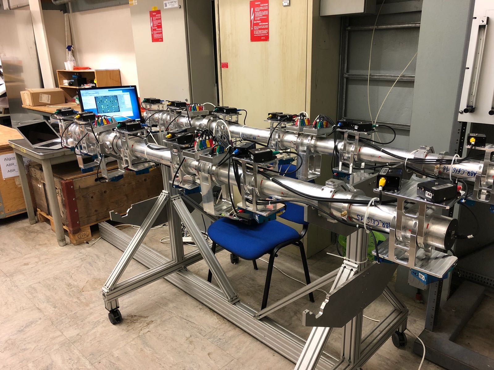
BCAM users, unlike astronomers, do not have to contend with the curvature of the earth. Nevertheless, if we are to combine the measurements made by two BCAMs into a more comprehensive measurement of the geometry of a structure, we must know the relative orientations of their mounting coordinates. Not only that, we must know the relative positions of their mounting coordinates, because BCAM sources, unlike stars, are not infinitely far away. One way to make sure we know the relative orientations and positions of two mount coordinate systems is to put both mounts on the same rigid plate, and measure the positions of the mounting balls. Another is to place many mounts upon a long flexible structure, measure their relative positions, and then monitor the shape of this flexible structure so as to determine any changes in the relative positions of the mounts. The alignment bars we designed for the ATLAS end-cap muon alignment system are examples of such flexible structures. The longest are aluminum tubes 9.6 m long and 85 mm in diameter.
A large BCAM system might consist of hundreds of BCAMs mounted upon a large structure, plus hundreds more mounted in groups upon rigid plates and flexible reference structures. The measurements of all BCAMs combined provides us with the geometry of the large structure in a single, global coordinate system. The measurements made by the BCAMs are similar to those made by theodolites, and combining their measurements is akin to triangulation. Unlike theodolites, however, BCAMs take their measurements quickly and automatically. A BCAM system provides a real-time picture of the shape of a large structure. BCAMs are small enough to be inserted into small spaces, and to look down narrow corridors.
Each BCAM provides two light sources. When a BCAM camera sees two light sources on another BCAM, the camera can measure the range of the two light sources, and also their rotation about the line joining the two BCAMs. The range is d/β, where d is the separation of the two sources and β is the angle they subtend at the camera. The rotation of the light sources is the same as the rotation of the line joining the sources in the camera image. We discuss the accuracy of these two measurements below.
[12-JUL-16] We use three coordinate systems in BCAM geometry calculations. They are image coordinate, mount coordinates, and global coordinates. The global coordinate system is the one we use top define the positions of the BCAM mounting balls. We may have ten BCAMs mounted on our apparatus, each of which requires three mounting balls, and we define the positions of their centers in the global coordinate system. We may have measured all the spheres with a CMM, or we may provide approximate locations for the mounting balls, sufficient to allow us to measure the displacement of objects from their initial positions.
The centers of the steel balls in each kinematic BCAM mount define its mount coordinate system, which we refer to as the bcam coordinate system in our code. The three balls on the mount fit into the three depressions beneath the BCAM. We make the balls after the shape of the depression, so the balls are called the cone, slot, and flat balls. The origin of mount coordinate is the center of the cone ball. The relative positions of the balls on an ideal mounting plate are given by the drawing below. But the BCAM is tolerant of balls that are up to 250 μm away from their nominal positions.

We must define the mount coordinate system in such a way that our calibration constants do not change when we move a BCAM from one mount to another, even if the balls in the second mount are 250 μm away from their relative positions in the first mount. For example, if the BCAM pivot point, which is close to the center of its camera aperture, is at position (20 mm, 10 mm, 0 mm) in one mount, it must be in the same position in a second mount, even if the separation of the slot and cone balls is 250 μm more or less, and the separation of the flat and slot balls is 250 μm more or less. We satisfy this criterion, and place the z-axis of the mount coordinate system approximately parallel to the camera axis with the following definition. The center of the cone ball is the origin. The cross product of the flat-cone and slot-cone vectors defines the y-axis. The z-axis lies in the plane of the three balls, and subtends a fixed angle of 0.2798 radians (16.031 degrees) with the slot-cone line. If the mounting balls are in their nominal positions exactly, then the z-axis bisects the angle subtended by the slot and flat at the cone, and points straight forward out of the BCAM, parallel to the sides of the chassis. The x-axis completes a right-angled coordinate system with the y and z-axes.
All of the computaionally intensive calculations required by BCAM image analysis and geometry are performed by our lwdaq library, which we compile from Pascal source code with the Free Pascal Compiler. You will find BCAM-specific geometry routines in bcam.pas, general-purpose geometry routines in utils.pas, and image analysis routines in spot.pas. Here is the routine from bcam.pas that calculates the location and orientation of a BCAM mount coordinate system from the global coordinats of its mounting balls.
{
	bcam_coord_from_mount takes the global coordintes of the camera mounting
	balls and calculates the xyz location and xyz rotation that together make up
	the pose of the mount coordinate system in global coordinates.
}
function bcam_coord_from_mount(mount:kinematic_mount_type):xyz_pose_type;

var
	origin,x_axis,y_axis,z_axis:xyz_point_type;
	c:xyz_pose_type;
	cs,cp,cs_normal:xyz_point_type;

begin
	with mount do begin
{
	The unit vectors cs and cp define a plane. The normal to this plane is the
	y-axis of the bcam coordinate system, as defined by the cross product of cp
	with cs.
}
		cs:=xyz_unit_vector(xyz_difference(slot,cone));
		cp:=xyz_unit_vector(xyz_difference(flat,cone));
		y_axis:=xyz_unit_vector(xyz_cross_product(cp,cs));
{
	The orientation of the bcam camera around its y-axis is set by the slot and
	cone. We create the z-axis of the bcam system by rotating sc by z_angle
	about the y-axis. The resulting z-axis lies parallel to the nominal optical
	axis of the camera. To perform the rotation, we define cs_normal using cs
	and y_axis.
}
		cs_normal:=xyz_unit_vector(xyz_cross_product(cs,y_axis));
		z_axis:=
			xyz_unit_vector(
				xyz_sum(
					xyz_scale(cs,-cos(bcam_z_angle)),
					xyz_scale(cs_normal,-sin(bcam_z_angle))));
{
	The x-axis is the cross product of the y and z axes respectively.
}
		x_axis:=xyz_unit_vector(xyz_cross_product(y_axis,z_axis));
{
	We place the origin at the center of the cone ball.
}
		origin:=cone;
	end;
{
	Compose the pose of the coordinate system.
}
	c.location:=origin;
	c.orientation:=
		xyz_rotation_from_matrix(
			xyz_matrix_from_points(x_axis,y_axis,z_axis));
	bcam_coord_from_mount:=c;
end;
The following figure illustrates the mount coordinate system for the Blue A-BCAM.

The y-axis of the mount coordinates for our black BCAMs point up from the base of the BCAM to the top of the BCAM. But in our blue BCAMs, the chassis is a mirror image of the black chassis, so that the slot and flat balls are swapped. Consequently, the y-axis in a blue BCAM points downwards.
The origin lies in the same place from one mount to the next provided that the diameters of the cone balls in each mount are the same. The absolute diameter of the kinematic mounting balls should be 6.35 mm ±10 μm. These are tight tolerances, but precision steel balls are inexpensive and readily available. These quarter-inch diameter balls are, however, hard to find outside the United States. If you need some, get in touch with us and we will figure out how to supply you with them.
The orientations of the mount coordinates with respect to the BCAM chassis will be fixed provided the slot under the BCAM points exactly at the cone, the flat is perfectly flat, and the balls have the same diameter. The variation between the diameters of the mounting balls should be ±2 μm. The accuracy of the slot and flat restrict the total deviation of the kinematic mounting balls from their nominal positions. As we mentioned above, we can tolerate no more than ±250 μm deviation from the nominal ball positions.
Locations on the surface of an image sensor we specify in image coordinates. The BCAM Instrument in our LWDAQ software returns spot positions in image coordinates. You can apply the BCAM analysis to an image of your own with the LWDAQ library command lwdaq_bcam. We describe the spot-finding analysis routine in more detail below. You will find a thorough description and illustration of image coordinates as they apply to the TC255 sensor surface in the TC255 Minimal Head Manual (A2016), for the TC237B in our TC237B Minimal Head Manual (A2070), and for the ICX424 in our Laboratory Camera Head Manual (A2075).

The diagram does not show the kinematic mounts beneath the BCAMs, but the figure above does. Looking at the diagram, the flat is at the rear right in the black BCAMs, and at the rear left in the blue BCAMs. In all cases, the flat is in the positive mount-coordinate x-direction with respect to the slot.
To obtain a line in global coordinates from a BCAM measurement position, we combine the BCAM's calibration constants in mount coordinates, the spot position in image coordinates, and the mounting ball positions in global coordinates.
First we transform the two-dimensional image-coordinate spot position into a three-dimensional mount-coordinate spot position. Our calibration constants tell us the bearing of the line joining the center of the image sensor and the camera pivot point. The center of the image sensor is not the image coordinate origin. It is a point in image coordinates we pick in our definition of image coordinates. Our definition is buried within our BCAM calibration code, bcam.pas.
const
  bcam_tc255_center_x=1.720;{along image coordinate x-axis (mm)}
  bcam_tc255_center_y=1.220;{along image coordinate y-axis (mm)}
  bcam_icx424_center_x=2.590;{along image coordinate x-axis (mm)}
  bcam_icx424_center_y=1.924;{along image coordinate y-axis (mm)}
Our routine for converting between image coordinates and mount coordinates is as follows. Note that our code refers to mount coordinates as bcam coordinates. The routine uses all the calibration constants in its calculation.
{
  bcam_ccd_center calculates the bcam coordinates of the ccd center.
}
function bcam_ccd_center(camera:bcam_camera_type):xyz_point_type;
begin
  with camera do
    bcam_ccd_center:=xyz_sum(pivot,xyz_scale(axis,-ccd_to_pivot));
end;

{
  bcam_from_image_point converts a point on the ccd into a point in bcam coordinates.
  The calculation takes account of the orientation of the ccd in the camera.
}
function bcam_from_image_point(p:xy_point_type;camera:bcam_camera_type):xyz_point_type;

var
  q:xy_point_type;
  r:xyz_point_type;
  cc:xyz_point_type;

begin
  cc:=bcam_ccd_center(camera);
  with camera do begin
    if code=bcam_icx424_code then begin
      q.x:=p.x-bcam_icx424_center_x;
      q.y:=p.y-bcam_icx424_center_y;
    end else begin
      q.x:=p.x-bcam_tc255_center_x;
      q.y:=p.y-bcam_tc255_center_y;
    end;
    if axis.z>0 then begin
      r.x:=cc.x+q.x*cos(ccd_rotation)-q.y*sin(ccd_rotation);
      r.y:=cc.y+q.y*cos(ccd_rotation)+q.x*sin(ccd_rotation);
    end else begin
      r.x:=cc.x-q.x*cos(ccd_rotation)+q.y*sin(ccd_rotation);
      r.y:=cc.y+q.y*cos(ccd_rotation)+q.x*sin(ccd_rotation);
    end;
    r.z:=cc.z;
  end;
  bcam_from_image_point:=r;
end;
Once we have the spot position in mount coordinates, we define a line in mount coordinates using our spot position and the calibrated pivot point position. We transform this line from mount coordinates into global coordinates using the global coordinates of the mounting balls. The global_from_bcam_line does this job in our code.
You don't have to compile and call our Pascal code to have access to these routines. We provide access to them for you through the LWDAQ software's TCL/TK interpreter. You can transform a spot position into a mount coordinate line using bcam_source_bearing. If you know the range of a light source, you can determine its position in mount coordinates in one jump using bcam_source_position. You can transform from mount to global coordinates with global_from_bcam_point and back into mount coordinates with bcam_from_global_point. If you want to predict the location of spots on the image sensor, you can use bcam_image_position. We use some of these routines in our granite beam calibration script, which we used to calibrate BCAMs on a granite beam with a straight edge, instead of with our roll-cage.
[12-JUL-16] Here we describe how we calibrate BCAM cameras and sources. We describe the calibration of source plates, which are BCAMs without cameras, in Source Plates. For all such calibrations, we use the BCAM Calibrator Tool and re-calculate sets of calibration constants with the BCAM Calculator Tool.

We express the properties of individual BCAMs in terms of mount coordinates. Thus the pivot point of the camera, which is the point through which all straight rays pass on their way to the image sensor, is given in mount coordinates, as is the direction of the optical axis.

Our camera calibration tells us the direction of each camera axis to better than 50 μrad with respect to its mount coordinates. Suppose we have two BCAMs on a rigid plate looking at two separate light sources. We have measured the plate exactly. We can now measure the angle subtended by the two light sources at some point on the plate close to the BCAMs. We measure the bearing of each source with respect to the pivot point of the camera that views it, and translate this bearing into a line in the coordinate system of the plate. The direction of each line will be correct to 50 μrad. We can therefore determine the angular separation of the two sources at a point in the plate to an accuracy of approximately 70 μrad.
The principle technique we use to calibrate BCAM cameras and sources is to mount the BCAM in a roll-cage and rotate it by 360° in 90° steps. We measure the positions of the mounting balls with respect to the base plate in all four roll-cage orientations using a CMM. Our CMM is accurate to ±2 μm. The CMM measurements give us the relative orientation and position of the mount coordinates in each orientation.
Camera calibration requires a source block. The source block consists of four lasers arranged in a square on a vertical plate and attached to an aluminum block. The block is such that when we press it up against a straight edge, and the roll-cage base up against the same straight edge, we find that the sources are centered on the field of view of a BCAM camera mounted in the roll-cage. We measure the dimensions and orientation of the shape made by the four lasers in the following way. We place the source block on the top surface of a micrometer stage. We bolt the micrometer stage to an optical table and view it with a BCAM at a range of around two meters. We move the source block 10 mm in 500-μm steps, perpendicular to the axis of the viewing camera. At each step we take an image of the four lasers in the source block. The known direction and length of the translation of all four lasers allows us to deduce their relative positions, and the orientation of their relative positions with respect to the optical table.

During camera calibration, we take an image of the source block from each of the four orientations of the roll-cage, and at two different ranges. From these eight images we obtain thirty-two spot positions, and from these thirty-two spot positions. We combine the spot positions with our measurement of the roll-cage and source block, and so obtain, with ample redundancy, the seven calibration parameters of the camera.

We summarize the measurements of the roll-cage and source block in apparatus measurements such as the following, which is the entry for the Black P-BCAM front camera calibration. We store the apparatus measurements in our apparatus database.
apparatus_measurement:
calibration_type: black_polar_fc
apparatus_version: BND7 {black and silver roll cage}
measurement_time: 20060518174500
operator_name: Kevan
data:
	57.715 53.969 -98.384 {0 degree cone}
	36.698 53.941 -171.387 {0 degree slot}
	78.659 54.061 -171.418 {0 degree flat}
	105.308 76.783 -98.316 {90 degree cone}
	105.352 55.725 -171.306 {90 degree slot}
	105.235 97.685 -171.361 {90 degree flat}
	82.485 124.376 -98.374 {180 degree cone}
	103.568 124.379 -171.357 {180 degree slot}
	61.608 124.260 -171.426 {180 degree flat}
	34.942 101.574 -98.258 {270 degree cone}
	34.968 122.615 -171.254 {270 degree slot}
	35.067 80.653 -171.3 {270 degree flat}
	1207.5 {range_1}
	2434.8 {range_2}
	80.2569 96.8127 {top-left laser}
	60.2921 96.8570 {top-right laser}
	60.2698 81.7400 {bottom-right laser}
	80.2576 81.7995 {bottom-left laser}
	+1 {axis_direction}
end.
We record the calibration measurements in device calibrations, which we store in our calibration database.
device_calibration:
device_id: 20MABNDL000099
calibration_type: black_polar_fc
apparatus_version: BND1
calibration_time: 20020819140700
operator_name: Michael
data:
1498.540 472.530 2659.530 459.540 2661.680 1330.130 1501.700 1343.970
1661.350 1445.440 1647.990 284.730 2518.890 282.290 2531.890 1442.460
2643.130 1294.030 1482.100 1306.690 1479.290 436.300 2639.550 422.910
2471.770 314.630 2485.230 1475.690 1614.480 1478.830 1600.270 317.760
1762.110 677.580 2360.530 670.190 2362.120 1119.360 1764.390 1126.830
1845.140 1178.150 1838.620 579.150 2287.120 577.500 2294.540 1175.520
2355.220 1105.500 1757.110 1112.210 1755.680 663.230 2353.240 655.970
2264.600 598.370 2271.340 1197.050 1822.570 1198.050 1815.190 600.730
end.
Source calibration requires a reference camera. We construct this camera out of a calibrated BCAM camera and an aluminum block. The sources of the camera need not be calibrated. The aluminum block is such that when we press the block up against a straight edge, and the roll-cage base plate up against the same straight edge, we find that the the sources of a BCAM mounted in the roll cage are in the center of the field of view of the reference camera. We measure the magnification and orientation of the image obtained by the reference camera in the following way. We remove the roll-cage and replace it with a BCAM mounted upon a micrometer stage. We take care to measure the range of the BCAM sources from the reference camera pivot point. We know the reference camera pivot point because we have already calibrated this camera using the roll-cage and source block. We move the BCAM sources 10 mm in 500-μm steps. The known direction and length of movement of the two sources gives us the magnification and orientation of the reference camera image at the known range of the two sources. We adjust our magnification from this measured value to suit the slightly different ranges of the various types of BCAM in the roll-cage.
During source calibration, we mount the BCAM in the roll-cage and take images of the sources with the reference camera in all four roll-cage orientations. From the four images we obtain eight spot positions. We combine these eight spot positions with our measurement of the roll-cage and calibration of the reference camera, and so obtain, with ample redundancy, the positions of both sources.
Here is the apparatus measurements for the calibration of Blue A-BCAM sources.
apparatus_measurement:
calibration_type: blue_azimuthal_s
apparatus_version: BND7 {black and silver roll cage}
measurement_time: 20060518174500
operator_name: Kevan
data:
	57.661901 76.205988 -189.557165 {0 degree cone}
	78.575848 76.314832 -262.605013 {0 degree slot}
	36.615268 76.130827 -262.566267 {0 degree flat}
	83.091621 76.679415 -189.489985 {90 degree cone}
	82.996787 97.550804 -262.550024 {90 degree slot}
	83.177793 55.590240 -262.486798 {90 degree flat}
	82.619448 102.107918 -189.535124 {180 degree cone}
	61.769633 101.973046 -262.601260 {180 degree slot}
	103.730167 102.156056 -262.525744 {180 degree flat}
	57.234556 101.644838 -189.415420 {270 degree cone}
	57.381470 80.756333 -262.470481 {270 degree slot}
	57.218463 122.716984 -262.417200 {270 degree flat}
	1.15 {mrad viewing_x_direction (needs to be checked)}
	18.564 {mm/mm viewing_scale}
	0.36 {bcam_front_source_z (mm in bcam coords)}
end.
Here is the device calibration for a pair Blue A-BCAM sources.
device_calibration:
device_id: 20MABNDB000101
calibration_type: blue_azimuthal_s
apparatus_version: BND7
calibration_time: 20061005135146
operator_name: Kevan
data:
1966.99 1266.88 1103.68 1271.05
1510.45 844.34 1514.47 1707.63
1089.30 1301.13 1951.83 1297.25
1546.85 1722.12 1542.91 860.00
end.
We describe the geometric calculations we use to obtain the calibration constants from the roll-cage measurements in the comments of our source code, bcam.pas, in particular the bcam_pair_calib procedure. The calibration calculation is available in the LWDAQ software through the lwdaq_calibration command.
Here are the calibration constants of a Black P-BCAM camera, all on one line:
12.747 35.282 3.705 2.115 -5.303 1 76.124 12.921
The first three numbers are pivot.x, pivot.y, and pivot.z. These are the x, y, and z mount coordinates of the camera pivot point, in millimeters. The next three numbers are axis.x, axis.y, and axis.z. These form a unit vector along the camera axis in mount coordinates, except that axis.x and axis.y have been multiplied by 1000 with respect to axis.z. Another way of thinking of these three constants is that they are the direction cosines of the camera axis, with axis.x and axis.y multiplied by a thousand. A third way of thinking about it, which is the one we use, and which explains why we give the units of x and y as milliradians, is that axis.x and axis.y are the angles the camera axis makes with the z-axis when projected into the x-z plane and the y-z plane respectively.
Example: At the point (pivot.x, pivot.y, pivot.z + 1000 mm) the shortest vector to the camera axis is (axis.x, axis.y, 0).
We try to make our BCAMs so that the axis direction lies within ±5 mrad of the z-axis, so |axis.x| < 5 mrad and |axis.y| < 5 mrad. The sixth number, axis.z gives the camera z-direction and the camera type, as shown below.
| axis.z | camera types (image sensor) |
|---|---|
| +1 | TC255 front-facing camera, A and P-BCAMs |
| −1 | TC255 rear-facing camera, P-BCAMs |
| +2 | ICX424 front-facing camera, H, N, and D-BCAMs |
| −2 | ICX424 rear-facing camera, H and D-BCAMs |
The seventh number, ccd_to_pivot, is the distance backwards along the camera axis from the pivot point to the surface of the image sensor, in millimeters. The final number, ccd_rotation, is the rotation of the image sensor about the camera axis in milliradians. Positive rotation is anti-clockwise when looking from the pivot point to the image sensor.
Here are the calibration constants from a Blue A-BCAM.
-12.677 -13.069 0.922 -2.249 -1.498 1 75.137 5.902
As you can see, the x and y coordinates of the pivot point position are both negative. The y-coordinate points downwards on the blue BCAM, but and the x-coordinate points the opposite direction from that of the black BCAM x-axis. Because the pivot point is on the other side of the cone ball in the blue BCAM, its x-coordinate is also negative. The distance from the pivot point to the image sensor is still positive, because we define this as positive when we move back along the camera axis to the image sensor, not when we move in any particular direction along the z-axis.
Here is the full output from our calibration program for the same Blue A-BCAM.
Calibration Constants for Front-Facing Camera on Device 20MABNDB000025:
 -----------------------------------------------------------------------
          |      Pivot Position   |   Axis Direction  |  CCD  |  CCD
          |-----------------------|-------------------| -to-  |  Rot-
          |    x  |   y   |   z   |    x  |    y  |   | Pivot |  ation
    Pair  |  (mm) |  (mm) |  (mm) | (mrad)| (mrad)| z |  (mm) |  (mrad)
 -----------------------------------------------------------------------
       1_2 -12.653 -13.078   0.698  -2.265  -1.497   1  75.143    5.795
       1_3 -12.684 -13.080   1.194  -2.227  -1.506   1  75.106    6.033
       1_4 -12.688 -13.076   1.306  -2.280  -1.500   1  75.116    6.014
       2_3 -12.686 -13.048   0.539  -2.232  -1.545   1  75.158    5.790
       2_4 -12.670 -13.059   0.651  -2.271  -1.491   1  75.169    5.771
       3_4 -12.679 -13.075   1.147  -2.219  -1.452   1  75.131    6.010
 -----------------------------------------------------------------------
   average -12.677 -13.069   0.922  -2.249  -1.498   1  75.137    5.902
    spread   0.036   0.032   0.767   0.061   0.093   0   0.063    0.262
     limit   0.080   0.080   4.000   0.100   0.100   0   0.300    1.000
 -----------------------------------------------------------------------
Calibration performed at time 20031031160639
We get six pairs of roll-cage orientations from our four orientations, and each pair gives us a set of calibration constants. The final calibration constants we provide for each BCAM are the average of the six values. We check the spread in calibration constants across these six pairs of orientations to see if anything went wrong while we were taking measurements and moving the calibration pieces. If the spread exceeds the limits, we print a warning line. The limits for each calibration parameter are defined in the bcam_camera_limit string in bcam.pas. Another string sets the limits for pairs of sources on BCAMs, which we discuss below.
bcam_camera_limit='limit 0.08 0.08 4 0.1 0.1 0 0.3 1';
bcam_sources_limit='limit 0.08 0.08 0.08 0.08 0.1';
In addition to checking the spread of values, we also check whether the average value for each constant lies within an acceptable range of the nominal values for the camera. The acceptable range is defined in the bcam_camera_range string of bcam.pas.
bcam_camera_range='range 1 1 10 10 10 0.1 2 100';
bcam_sources_range='range 1 1 1 1 0.1';
Here are the source calibration constants for a Blue A-BCAM.
Calibration Constants for Front Sources on Device 20MABNDB000025:
 -------------------------------------------------
          | First Source  | Second Source |
          |-----------------------|-------|
          |   x   |   y   |   x   |   y   |   z
    Pair  |  (mm) |  (mm) |  (mm) |  (mm) |  (mm)
 -------------------------------------------------
       1_2 -20.644 -13.088  -4.634 -13.051   0.360
       1_3 -20.647 -13.083  -4.655 -13.050   0.360
       1_4 -20.639 -13.066  -4.639 -13.051   0.360
       2_3 -20.642 -13.079  -4.654 -13.029   0.360
       2_4 -20.630 -13.079  -4.636 -13.048   0.360
       3_4 -20.631 -13.091  -4.655 -13.066   0.360
 -------------------------------------------------
   average -20.639 -13.081  -4.646 -13.049   0.360
    spread   0.017   0.025   0.022   0.037   0.000
     limit   0.040   0.040   0.040   0.040   0.040
 -------------------------------------------------
Calibration performed at time 20031031115752
The source positions are the centers of the transmitting facets of the lasers. We give the x and y coordinates of each laser, and then its nominal z-position. Our calibration procedure does not measure the z-position of the lasers, but we know by construction where they are to within ±50 um.
There are two ways to calculate the calibration constants. The fast method that is always used by the BCAM Calibrator, and is the default in the BCAM Calculator, calculates pivot.z using all possible pairs of sources at both ranges, then calculates ccd_to_pivot using pivot.z and all pairs of sources at the close range, then uses pivot.z and ccd_to_pivot to get pivot.x, pivot.y, axis.x, and axis.y in a series of pairings of roll cage orientations that use each source on its own at both ranges. The final calculation is rotation using the near range sources. The simplex method we turn on with the Simplex button in the BCAM Calculator. This method uses the simplex fitting algorithm to minimize the disagreement between the BCAM's measurement of source positions and our apparatus values for source positions. Not only does the simplex fitter adjust the BCAM calibration constants, but it also must adjust the x and y offset of the source block with respect to the roll cage coordinates at both the near and far ranges, making a total of eleven parameters to fit.

The simplex method agrees with the fast method with the exception or pivot.z, ccd_to_pivot, and ccd_rotation, where small disagreements arise. The simplex method is several orders of magnitude slower than the fast method. We use the simplex method to check the fast method.
[12-JUL-16] Here we provide tables of the nominal values for the BCAM calibration constants. These are the values the constants would have if a BCAM turned out exactly as specified in our drawings.
-----------------------------------------------------------------------------
                |      Pivot Position   |   Axis Direction  |  CCD  |  CCD
                |-----------------------|-------------------| -to-  |  Rot-
                |    x  |   y   |   z   |    x  |    y  |   | Pivot |  ation
   Type         |  (mm) |  (mm) |  (mm) | (mrad)| (mrad)| z |  (mm) |  (mrad)
-----------------------------------------------------------------------------
black_azi_c      -12.675  13.137   2.000   0.000   0.000   1  75.000   3141.6
blue_azi_c       -12.675 -13.137   2.000   0.000   0.000   1  75.000      0.0
black_polar_fc    12.751  35.311   2.000   0.000   0.000   1  75.000      0.0
black_polar_rc   -12.751  35.311 -81.900   0.000   0.000  -1  75.000      0.0
blue_polar_fc     12.751 -35.311   2.000   0.000   0.000   1  75.000   3141.6
blue_polar_rc    -12.751 -35.311 -81.900   0.000   0.000  -1  75.000   3141.6
black_h_fc        12.751  35.311   2.000   0.000   0.000   2  50.000      0.0
black_h_rc       -12.751  35.311 -81.900   0.000   0.000  -2  50.000      0.0
blue_h_fc         12.751 -35.311   2.000   0.000   0.000   2  50.000   3141.6
blue_h_rc        -12.751 -35.311 -81.900   0.000   0.000  -2  50.000   3141.6
black_n_c        -10.439  21.666   0.000   0.000   0.000   2  49.2        0.0
blue_n_c         -10.439 -21.666   0.000   0.000   0.000   2  49.2     3141.6
black_d_fc        12.675  39.312   1.1     0.000   0.000   2  48.5        0.0
black_d_rc       -12.675  39.312 -81.0     0.000   0.000  -2  48.5        0.0
blue_d_fc         12.675 -39.312   1.1     0.000   0.000   2  48.5     3141.6
blue_d_rc        -12.675 -39.312 -81.0     0.000   0.000  -2  48.5     3141.6
-----------------------------------------------------------------------------
The table below gives the nominal source calibration constants for the existing BCAM cameras.
---------------------------------------------------------
                 | First Source  | Second Source |
                 |-----------------------|-------|
                 |   x   |   y   |   x   |   y   |   z
    Type         |  (mm) |  (mm) |  (mm) |  (mm) |  (mm)
---------------------------------------------------------
black_azi_s       -20.676  13.137  -4.764  13.137   0.36
blue_azi_s        -20.676 -13.137  -4.764 -13.137   0.36
black_polar_fs      4.674  36.812  20.670  36.812   0.36
black_polar_rs     -4.674  36.812 -20.670  36.812 -82.85
blue_polar_fs       4.674 -36.812  20.670 -36.812   0.36
blue_polar_rs      -4.674 -36.812 -20.670 -36.812 -82.85
black_h_fs          4.674  35.311  20.670  35.311   0.36
black_h_rs         -4.674  35.311 -20.670  35.311 -82.85
blue_h_fs           4.674 -35.311  20.670 -35.311   0.36
blue_h_rs          -4.674 -35.311 -20.670 -35.311 -82.85
black_n_s         -18.440  21.666  -2.438  21.666  -0.64
blue_n_s          -18.440 -21.666  -2.438 -21.666  -0.64
black_d_fs          4.674  39.312  20.670  39.312   0.30
black_d_rs         -4.674  39.312 -20.670  39.312 -80.21
blue_d_fs           4.674 -39.312  20.670 -39.312   0.30
blue_d_rs          -4.674 -39.312 -20.670 -39.312 -80.21
---------------------------------------------------------
In each case, we refer to "first source" and "second source". Each source has associated with it a device element, which we use to specify the source in our LWDAQ Software. For the front sources of all BCAMs, the first source is device element number three (ON3) and the second is number four (ON4). For the rear sources, the first source is element number one (ON1) and the second is two (ON2).
| Name (Letter Origin) | Front Center Laser |
Front Outer Laser |
Rear Center Laser |
Rear Outer Laser |
Front Camera |
Rear Camera |
|---|---|---|---|---|---|---|
| A-BCAM-L (Black Azimuthal) | 4 | 3 | None | None | 1/2 | None |
| A-BCAM-R (Blue Azimuthal) | 4 | 3 | None | None | None | 1/2 |
| P-BCAM-L (Black Polar) | 3 | 4 | 1 | 2 | 2 | 1 |
| P-BCAM-R (Blue Polar) | 3 | 4 | 1 | 2 | 2 | 1 |
| H-BCAM-L (Black High-Profile) | 3 | 4 | 1 | 2 | 2 | 1 |
| H-BCAM-R (Blue High-Profile) | 3 | 4 | 1 | 2 | 2 | 1 |
| N-BCAM-L (Black New Small Wheel) | 4 | 3 | None | None | 1/2 | None |
| N-BCAM-R (Blue New Small Wheel) | 4 | 3 | None | None | 1/2 | None |
| D-BCAM-L (Black Double-Ended) | 3 | 4 | 1 | 2 | 2 | 1 |
| D-BCAM-R (Blue Double-Ended) | 3 | 4 | 1 | 2 | 2 | 1 |
The table above associates the element numbers with locations on the chassis. The first sources are element numbers are 1 or 3 and the second sources are element numbers 2 or 4.
A BCAM can measure the absolute bearing of a light source, track the angular movement of a light source, measure the range of a pair of light sources, and measure the rotation of a pair of light sources. We consider each of these measurements in turn.
[12-JUL-16] The absolute accuracy of a BCAM is dominated by the accuracy of its calibration, which is usually 30 μrad rms, but is guaranteed to be better than 50 μrad rms. Assuming we know exactly where its mounting balls are, a BCAM will measure the bearing of a source to within 50 μrad rms. Two or more BCAMs can obtain an absolute measurement of a source position by triangulation, in which the bearings of a source from two different and well-known locations are combined to obtain its position. If two BCAMs are looking at the same source from two directions 90° to one another, both 10 m from the source, the two BCAMs determine the location of the source in three dimensions with an absolute accuracy of 500 μm rms. At range 1 m, the accuracy is 50 μm. At closer ranges, we must consider the accuracy with which we know the location of the pivot point, which is around 10 μ rms, and add this uncertainty to our error calculation.
The angular resolution of a BCAM camera 5 μrad or better at all ranges. Its resolution when measuring a small angular separation is therefore √2 × 5 μrad = 7 μrad. If we want to measurement of a large angular separation, we must rely upon the accuracy of scaling factor that relates the angular separation of source points to the separation of their images on the image sensor. This scaling factor is represented in our camera calibration constants as the distance between the pivot point and the image sensor. Our camera calibration gives us this distance to better than one part in a thousand (0.1%). If the angular separation of two sources is 10 mrad, our accuracy is 10 μrad, and our resolution is 7 μrad.
Now let us consider how well the BCAM can measure the co-linearity of three points. We have a camera at one of the extreme points looking at sources at the other two points. We measure the size of the angular separation of these sources with resolution 7 μrad and accuracy 0.1%. But there are other sources of error in our co-linearity measurement. To make sense of our angular measurements, we must also know the location of the camera pivot point with respect to its mount, and the locations of the two light sources with respect to their mounts. Then we can say that we are measuring the co-linearity of the three mounts. The co-linearity measurement therefore depends upon the accuracy with which we know the position of the pivot point in the directions perpendicular to the camera axis, and the positions of the sources in the same directions. Our calibration tells us the pivot point position to better than 20 μm in the directions perpendicular to the camera axis, and the source positions to better than 10 μm.
[12-JUL-16] Because we know the separation of BCAM light sources in a BCAM chassis, we can measure the distance between two BCAMs by measuring the angle subtended by these sources at the viewing camera.

The range is equal to the separation of the lasers, d, divided by the angle they subtend, β.
r = d/β,
The sensitivity of measured range to angular separation is given by,
dr/dβ = −d/β2 = −r2/d.
As the range increases, the subtended angle decreases, so that the error in our range measurement increases as the square of the range. If the error in measuring changes in the bearing, α, of a single source is σ(α), our error in measuring the angular separation of two light sources, σ(β), is √2 σ. Our error in measuring range is:
σ(r) = √2σ(α)r2/d.
Our BCAM sources are separated by 16 mm and calibrated to 10μm rms. The cameras measure bearing with 5 μrad rms precision. They measure range with error 2 mm at ranges close to 2 m and error 40 mm at ranges close to 10 m.
A BCAM can measure the rotation, θ, of another BCAM about the line joining the two. This rotation is the same as the rotation of the line joining the light sources images. Our error in measuring this rotation is,
σ(θ) = √2σ(α)/β = √2σ(α)r/d
At range 2 m, we measure the rotation with error 1 mrad. At range 10 m, our error is 4 mrad.
[11-APR-19] The BCAM sits upon three quarter-inch steel balls (diameter 6.35 mm). We hold it in place with a single M4 screw with 0.7-mm threads. The following table is a guide to the length of screw required by our various types of BCAM.

We secure our P-BCAMs with 50-mm screws, and our A-BCAMs with 40-mm screws. We like to provide at least 7 mm of thread in the mounting plate, which is 1.5× the screw diameter plus and extra millimeter. We recommend a minimum depth of 4 mm in aluminum, and 3 mm in steel. We recommend a hex head screw because it gives us better control when tightening the screw. As we tighten the screw, the ball beneath the flat depression of the kinematic mount bites into the flat, and we rotate the BCAM. The depth to which the mounting ball bites into the flat is proportional to the tension in the screw. The tension in the screw is proportional to the deformation of the BCAM lid beneath the screw head. The lid of the BCAM acts like a spring, moderating the force with which the enclosure is held to the mounting balls. Accurate calibration of the BCAM requires that we always mount it with the same screw tension as we used during calibration. With the same screw tension, we get the same rotation of the BCAM as the ball bites into the flat depression.
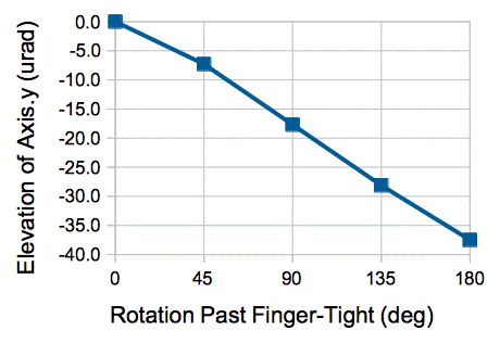
To secure the BCAM accurately, we insert an Allen key in the head of the mounting screw and tighten the screw by rotating the vertical shaft of the Allen key with finger and thumb. The screw is now finger-tight. Once the screw is finger-tight, we tighten it by one more quarter-turn, which pushes the lid down by 200 μm. The resulting indentation made in the flat depression by its mounting ball is roughly 500 μm in diameter, which means it is a 10 μm deep. As we force the BCAM down on onto the flat depression's ball, the BCAM chassis rotates about the line joining the cone and slot balls. This rotation has two effects upon our calibration constants. The image sensor rotates about the camera axis, and the camera axis itself tilts upwards. We measured the effect of tightening by an extra half-turn in Fastening Screw. We study the effect of dents in the slot and flat depressions in The Effect of Dents in the BCAM Kinematic Mount. Tightening by a half-turn in a Black A-BCAM tilts axis.y up by 20 μrad rotates the image sensor by 50 μrad. When we tighten the screw in steps on a Blue N-BCAM, we obtain the following change in axis.y with rotation of the screw.
We asked five different members of our group to follow a "finger-tight plus half-turn" mounting procedure. Each time we measured the bearing of a light source five meters away. The standard deviation of the bearing was 10 μrad. We concluded that the mounting force was consistent to within 10%. If we tighten the mounting screw "finger-tight plus one-turn", we make a 500-μm diameter depression in the flat surface that is 10 μm deep. We can loosen the screw by half a turn, but this depression will not go away. The BCAM will always mount incorrectly on this particular ball triplet and any other ball triplet that brings the flat ball into the 10-μm depression.
Nowadays, we use torque screw drivers to tighten BCAM screws in our laboratory. We tighten the screw to "twenty ounce-inches", which is 0.14 Nm. This torque is equal to the torque we obtain with finger-tight plus one quarter-turn. If we ignore friction between the screw and the lid, we see that this 0.14 Nm acting on the 0.8-mm threads generates a downward force of 1000 N, which would be like placing a 100-kg weight on the BCAM. But the force the screw generates in practice is far less than this. We can raise the BCAM up off its balls, while it is screwed down, by exerting a force of no more than 100 N. We conclude that friction between the screw and the lid play a critical role in moderating the fastening force, and we rely upon the consistency of this friction for the consistency of our mounting procedure.
Be sure to follow our finger-tight plus quarter-turn rule or use a torque screw driver set to 0.14 Nm when you fasten BCAMs to their mounts. Over-tightening the mounting screw will damage the BCAM. Both over-tightening and under-tightening will change both the image sensor rotation and axis direction of the BCAM's cameras. The calibration constants we provide apply to BCAMs secured to their mounts according to the finger-tight plus quarter-turn rule.
[12-JUL-16] A BCAM image is a photograph taken by a BCAM camera of one or more BCAM lasers. The simplest BCAM image capture procedure is as follows.
Background-subtraction image capture procedure is as follows.
We connect our BCAMs to LWDAQ Hardware. We control the hardware via TCPIP using the LWDAQ Software. If you want to write your own software to capture BCAM images, you will need to know the image captures steps in detail. Instead of describing the steps in detail here, we recommend that you look at BCAM.tcl. This file is a TclTk script. It declares the LWDAQ_daq_BCAM procedure, which defines the image capture process for the BCAM Instrument in our LWDAQ Software.
Our data acquisition software uses the LWDAQ to digitize BCAM images with eight-bit resolution. The pixel intensities range from zero to 255. When we subtract the background image, we may find that the result is slightly negative. Our electronically-generated image noise is a fraction of an ADC counts rms, but when there are sudden changes in the ambient light intensity, the background might be several counts brighter in places than the laser image. In some cases, with unshielded cables or damaged electronic circuits, we have observed noise spikes several counts high. Because we store these images as arrays of bytes in memory, the value −1 will be recorded as 255. Our analysis program simply sets negative values to zero.
Background subtraction does require us to capture two images from the BCAM, which doubles your data acquisition time. In our laboratory, we rarely use background subtraction, because we have no sunlight to worry about, and we like the data acquisition to be fast.
Whether an image is background-subtracted or not, we must check to make sure that its peak intensity lies within an acceptable range before we analyze the image to find the locations of its laser spots. We will talk more about the acceptable range of image intensities later, but for now, let us assume that we wish to capture a BCAM image with a peak intensity that lies between 100 and 140 counts above the average intensity in the image. If the peak intensity is too high, we must reduce the time for which we flash the laser, which we call the exposure time. Conversely, if the peak intensity is too low, we must increase the exposure time.
There are several other properties of the image we can check to make sure our image is useful and accurate. The figure below shows an example quality assurance procedure.

The light spots in most images take up only a small part of the entire image sensor. If we want to see what lies within the field of view, perhaps to determine whether our BCAM camera is facing in the right direction, we can capture an ambient image with a slightly different, and simpler, procedure.
The 100 ms of step (2) is the ambient-light exposure time. Here is an example ambient-light image.

You will notice the black band on the left side of the image. This band is made up of eighteen black columns. The first six of these columns are added to the image by our data acquisition hardware. The remaining twelve are black-level reference columns in the image sensor. The black-level are like any other columns in the image, except they are kept in the dark by a layer of aluminum. As you can see, the blue analysis boundary of Figures 4 and 5 excludes the first eighteen columns of the image.
An ambient-light image requires ambient light. If there is no ambient light, you can try to make your own by flashing one or both of the lasers on the BCAM that is taking the ambient-light picture. You might see something in the reflected light of the lasers. Unfortunately, because the lasers emit highly coherent light, an image obtained with their illumination will be plagued with bright and dark spots, or laser speckle.
You will find an example background-subtracted image above. If you would like to experiment with the BCAM software, you can use our demonstration stand to capture BCAM images.
[12-JUL-16] The standard deviation of intensity in this image is only four ADC counts. To display this image clearly, we intensified it. Our display programs provide three grades of intensification, each of which comes into its own for particular images. We will be glad to supply you with our intensification source code. We use exact intensification with images like this. Exact intensification shows the brightest spot in the analysis boundary as white, and the darkest spot as black. We have two other varieties of intensification, each of which uses the standard deviation of the image intensity within the analysis boundary, which we call the image amplitude, and the average intensity, which we call the image background to determine the display intensity. We displayed the ambient-light image above with mild intensification. With mild intensification, any pixel with intensity five or more amplitudes above the background appears white, and any pixel five or more amplitudes below background is black. With strong intensification we do the same, except with a limit of two amplitudes above and below the background.
[12-JUL-16] When a viewing BCAM monitors a light source on a target BCAM, we can rotate the viewing BCAM only by so much before the laser leaves the field of view, and we can rotate the target BCAM only by so much before the cone of light emitted by the light source no longer shines upon the viewing BCAM. The field of view of the camera is the angle by which we can rotate the camera and still view a stationary light source.
The A and P-BCAMs use the TC255 image sensor. The active area of this sensors is roughly 3.2 mm × 2.4 mm. The sensor is 75 mm from the camera pivot point. The field of view is a rectangular cone. The angle subtended by this cone is 43 mrad in the horizontal direction and 32 mrad in the vertical. So the field of view of the A and P-BCAMs is 43 mrad × 32 mrad. At range 10 m, the rectangular cone is 43 cm by 32 cm. We usually quote the field of view as 40 mrad × 30 mrad.
The H-BCAMs use the ICX424 image sensor. The active area of this sensor is roughly 5.1 mm × 3.8 mm. The sensor is a little less than 50 mm from the camera pivot point. The field of view is a rectangular cone slightly more than 101 mrad × 76 mrad at its base. At range 10 m, this cone is at least 100 cm by 76 cm, more than twice as wide as the field of view of the A and P-BCAMs. We usually quote the field of view as 100 mrad × 75 mrad.
The viewing angle of the laser is the angle over which we get more than 10% of the maximum light intensity from the laser. If you hold a piece of white paper 100 mm in front of a LDP65001E laser, it shines a bright stripe of light on the paper roughly 75 mm by 25 mm. The internal angles of the cone are roughly 40° and 14°. The following graph shows how the relative intensity of the light arriving from the laser varies with rotation about an axis parellel to the longer side of the laser stripe.

This graph shows a viewing angle of ±7°, which matches our 14° viewing angle in the narrow direction of the cone. Once we leave the viewing range, the intensity drops dramatically and we find that the center of the laser appears to move by tens of microns. For the BCAM to perform at its specified accuracy of 0.5 μrad resolution and 50 μrad absolute accuracy, we must ensure that the laser viewing angle includes the viewing camera pivot point.
[12-JUL-16] In Some Unoriginal Thoughts on Thermal Gradients and Turbulence in Air, we discuss the bending of light by static temperature gradients and the displacement of light by bubbles of lighter or heavier air. The errors caused by static gradients can be large. The errors caused by moving bubbles of air are smaller and random. In almost all BCAM applications, performance of the BCAMs is improved by the introduction of fans to blow air around. When air is turbulent, it cannot build up static gradients that bend light, and the bubbles of differing density that the turbulent air contains are smaller than those in slow-moving air.
Suppose we are working on a granite table. We have the lights on overhead. We arrange BCAMs on the smooth surface so that they face one another. We leave the table and the BCAMs alone for a few hours. We record spot positions on the BCAM image sensors. When we return, we find that the table has apparently bent in our absence. We turn on a fan and keep taking measurements. Now the table appears to un-bend immediately. The apparent bending cannot be real because the granite table is large and heave and takes a long time to cool down and straighten. The apparent bending is due to a temperature gradient perpendicular to the table surface, and therefore perpendicular to the BCAM optical paths.
The granite table is being heated by our overhead lights. The air in contact with it is warmer than the air higher up. The temperature difference is slight. It is insufficient to start a process of convection. As we show in our talk, the displacement, a, of a light ray by a gradient dT/dx perpendicular to the light ray is:
a = l 2(dT/dx) × 0.5 μm K−1m−1
Along a 4-m table with 10 K/m vertical gradient, we get a total displacement of 80 μm along an arc. As the ray enters the lens of a BCAM, its bearing is changed by 2 × 80 μm / 4 m = 40 μrad, which is much larger than the BCAMs resolution of 5 μrad. A temperature gradient of 10 K/m is only 0.3 K in the 3 cm height that is likely to contain a BCAM optical path. In our experience, it is easy to develop such gradients with overhead fluorescent lighting.
When we turn on a fan, the static thermal layer is destroyed, and we see no systematic displacement of the BCAM image. Instead, we see random movements of the spot caused by moving bubbles of air of different density. In our experience, these errors are of order 2 μrad rms when we have a fan blowing over a granite surface.
When you are working close to horizontal surfaces, use fans to obtain accurate measurements.
If we don't want fans, we should place our BCAM optical paths far above horizontal surfaces, or arrange for the BCAM optical paths to lie between vertical surfaces, or far from any surface that might develop a static temperature gradient perpendicular to the optical path. In the ATLAS experiment for which we designed the BCAM, we have no optical paths along horizontal surfaces.
When we are far from static gradients, but operating without the benefit of fans, the random errors caused by slow-moving bubbles of air are larger. At range 4 m in our laboratory, we will often see atmospheric errors of order 5 μm. We designed the BCAM so that the errors introduced by its optics, chassis, and electronics are less than the 5 μm error we expect from turbulence in open-air applications without fans.
[12-JUL-16] Ambient illumination is rarely a problem with BCAM cameras, because the field of view is so small and the lasers are so bright. But there are times when it is a problem, especially when sunlight is reflecting into the BCAM field of view, as shown in below.

When an ambient light or a reflection of ambient light does appear in the field of view, our analysis program cannot distinguish between the laser and the reflection. If there is a steady gradient to the ambient illumination across the field of view, the apparent position of the laser image will be displaced in the direction of the gradient.
We can remove ambient light from our final image, so long as it is the ambient light is not so bright as to saturate our image sensor. We capture two separate images, one with the lasers flashing, and the other with the lasers off. The second image is our background image. We subtract the background from the image we take with the lasers flashing, to obtain our final image. We call this procedure background subtraction, and we use it whenever we have problems with ambient light.
[12-JUL-16] A synchronous reflections is a reflection of the light source off some shiny surface in the field of view of the BCAM. Unlike ambient light, reflections of the lasers cannot be removed from our final image by background subtraction. The reflections are present if and only if the lasers are flashing. The brighter the lasers, the brighter the reflections. We call them synchronous reflections because they occur whenever we flash the light source.
It is usually true that the BCAM's direct view of a light source is brighter than any of its reflected views of the same source. Thus we can usually eliminate reflections by sorting all the spots in the image into decreasing order of brightness, and taking the first one. But there are certain circumstances in which the reflections will be brighter than the direct view. When looking down the center of an aluminum tube, a light source at the far end can be reflected by the curving walls of the tube so as to create a large image with greater total brightness than the direct view.
It is almost always true that the direct view will have greater peak brightness than any reflection. We can be more certain of eliminating reflections if we sort in order of decreasing peak intensity. But even this method does not guarantee that we eliminate synchronous reflections. Looking down the center of a shiny tube, the intensity at the center of a sharply-focused direct spot may be greater, but when spread over the pixel, it can be less than the intensity of the brightest pixel in a reflected image off the tube walls. Synchronous reflections off the inner walls of tubes cause such problems with image analysis that we have yet to succeed in implementing a BCAM system within a tube, although such a system is in principle possible.
[12-JUL-16] Suppose we cover our BCAM with a black cloth and take an ambient-light image with a zero-second exposure time. The amplitude of this image is what we call the image noise. You can learn more about the nature of the noise in an image by displaying the blank image with intensification. You should see randomly-scattered points of bright and dark, with image amplitude between 0.1 and 1.0 ADC counts, depending upon the length of your cables and their environment. In theory, when we digitize an image pixel with our eight-bit ADC, we introduce quantization noise of 0.3 counts rms. But if the image has uniform intensity, the quantization is smaller. The noise in our laboratory images is usually 0.2 counts, even with long cables coiled upon the floor. But the image noise in large data acquisition systems with long cables, such as ATLAS or ALICE, can be as high as 1.0 counts.

You might see noise that is not random, as in the image above. Diagonal noise can be caused by switching power supplies.. In our experience, the intensity of diagonal noise is never more than 1 count, and has no significant affect upon the performance of a BCAM.
Far worse than diagonal noise are noise spikes. These appear as white and black pixels distributed randomly in the image. If their height is always less than ten or twenty counts, they are probably the result of damaged electronics in the BCAM camera or of a faulty cable. If their height ranges from one to one hundred counts, they are probably the result of noisy transmission between the LWDAQ driver and your data acquisition computer. Small noise spikes you can overcome, if you have to, by raising the analysis threshold. Large noise spikes make image analysis impossible. In either case, the noise spikes indicate that something is wrong with your data acquisition hardware.
[12-JUL-16] Our advertised 5-μrad source bearing resolution, requires us to measure the position of point source images with resolution 400 nm on the image sensor. (The image sensor is 75 mm from the pivot point, and 75 mm multiplied by 5 μrad is 375 nm.) In the P or A-BCAMs, this 400 nm is 4% of a pixel width. When the source is three meters from the BCAM, the image is only four pixels wide, so 400-nm is 1% of the image width.
The LWDAQ provides images with electronic noise less than 0.1% of the image intensity. Even the smallest images spread their light over twenty or thirty pixels, so when we calculate the light centroid we average the electronic noise over twenty or thirty pixels. It is not at first obvious that we can determine the position of a light spot to better than 4% of a pixel width. Nevertheless, with a simple weighted-centroid calculation, we can obtain 4% resolution or better, even with pixels that span only four pixels.
The BCAM Instrument captures BCAM images and analyzes them. It gives you a choice between single-spot or multi-spot analysis. In single-spot analysis, the BCAM Instrument assumes that there is only one spot, and it uses every pixel in the analysis boundaries to determine the location of the spot. In multi-spot analysis, the BCAM Instrument identifies connected groups of pixels above threshold, enclose each such group in a rectangle, and calculate the group's centroid using only the pixels within this rectangle.
If you look in the image above, or in images you take from our demonstration stand, you will see a blue rectangle that marks the analysis boundaries. We set the analysis boundaries to include however much of the image we want to use. The BCAM rejects spots outside the boundaries. Its multi-spot analysis returns a list of spots sorted in order of descending brightness. By flashing one laser in the field of view, and choosing the brightest spot returned by the analysis, the BCAM allows you to reject reflections and noise.
If you want to look at our BCAM image analysis code, you will find it in spot.pas. This source code is in Pascal, and compiles with the GNU Pascal Compiler. The code will show you how we use the image's analysis boundaries to restrict our analysis to pixels in a single rectangle, and how we find smaller rectangles that enclose individual spots within the analysis boundaries.
Our centroid-calculating routine subtracts a threshold from the intensity of each pixel associated with a spot, and calculates the weighted sum of the spot intensity after subtraction. Any pixel whose intensity is negative after subtracting the threshold we eliminate from the sum, by setting its intensity to zero. We recommend a threshold a few counts above the average image intensity, or that you calculate the threshold by examining the intensity of the image. We obtain robust and accurate analysis by taking the average and maximum intensities in the image, and picking a threshold that is 10% of the way from the average to the maximum. The BCAM Instrument allows you to instruct the BCAM Instrument to perform this threshold determination automatically.
Here is the result of BCAM image analysis on the image shown above.
BCAM_1 2697.50 1413.94 22 210 0.003 58 1694.20 1401.24 26 202 0.001 58
The first two numbers are the position of the brightest spot, given in microns in image coordinates. The third number (22) is the number of pixels above threshold in the spot. The fourth number (210) is the total above-threshold brightness of all these pixels. The fifth number (0.003) is the change in spot position for a one-count increase in threshold. The sixth number (58) is the threshold used. The final six numbers have the same meaning, but apply to the second brightest spot in the image.
For more information on how to use the BCAM Instrument, see the LWDAQ User Manual. For a definition of the image capture procedure we use in our LWDAQ Software, see BCAM.tcl. In addition to the well-established centroid-finding routine, spot.pas provides a straight-line fit to the pixels in a spot, and an ellipse fit to the perimeter of a spot. These alternative spot-finding routines are useful in instruments such as the Wire Position Sensor, in which a wire edge appears as a stripe in a derivative image, or in a BCAM with large, retroreflecting targets instead of tiny laser light sources.
[12-JUL-16] The focal range of a BCAM is the range at which its image of a point source will be in the sharpest focus. A laser diode at the focal range will produce a smaller image than at any other range. The default focal range for P-BCAM, A-BCAM, D-BCAM, and N-BCAM cameras is 3 m. For H-BCAMs the default focal range is 1.5 m.

The size and shape of the laser images we see at range 3 m are a function of the optics of the camera only. With perfect lens and a large aperture, the image of a laser at the focal range would be a spot on the image sensor a few microns wide. But diffraction at the 2-mm aperture of the BCAM camera spreads the light spot until it covers several pixels, even when the image is in perfect focus. This radially-symmetric blurring of the spot allows us to measure the position of the spot with an accuracy of a fraction of a pixel width by taking the weighted centroid of the light intensity in the pixels. If the image were smaller than one pixel, we would be unable to detect its movement across the width of a pixel.
Diffraction: Rays passing through an aperture of diameter d spread out in a cone of angle λ/d, where λ is the wavelength of the light. The A and P-BCAMs have a 2-mm aperture and 75-mm distance from the aperture to the TC255 image sensor. Diffraction takes the image of a 650-nm red laser and spreads it to a diameter of 24 μm, or 2.5 of the sensor;s 10-μm pixels. A 470-nm blue fiber source will be spread to 18 μm. The H-BCAM and N-BCAM have a 2-mm aperture and 50-mm distance to the ICX424AL image sensor. A red laser image will be at least 16 μm across, or 2.2 of the sensor's 7.4-μm pixels. A blue fiber source image will be at least 12 μm wide.
At shorter ranges, the laser image grows as it becomes defocused. At around 60 cm, depending upon the BCAM, a black hole may appear in the middle. The black hole is the result of destructive interference at the center of the image. If we use incoherent, flat-topped infra-red light-emitting diodes as a light sources, we still see the same hole in the image. The hole is not a consequence of using a coherent laser light source. At longer ranges, the spot spreads out also, but not to the same extent. Images at ranges greater than ten meters all look the same. The only upper limit to the BCAM range is the camera exposure time required to obtain a clear image.

By default, we adjust the lenses of our BCAMs until a red laser at range 3 m has the smallest possible image diameter. Thus the focal range for red light is 3 m. But we can reduce the focal range by placing the lens farther from the image sensor. If we move the focal range of a P-BCAM to 1.5 m, images at 60 cm no longer show a black hole in the middle. But images at rangers greater than eight meters are a bright point in the middle, with a dark ring outside, and a dim ring farther out, as you can see below.
In the A and P-BCAMs, which both use the TC255 image sensor, the ten-meter image above produces errors of several microns in the measurement of the image location, as we describe at length in BCAM Focus. It turns out that there is a thin, dark circle of destructive interference around the bright center of the image spot. This dark circle is so thin that we cannot see it with our 10-μm pixels. If we move the light spot across the image sensor in uniform steps, we see cyclic non-linearity in our measurement of the image position. We suspect that these cycles are caused by regular features on the image sensor interacting with the thin, dark circle. Such non-linearity at long ranges introduces errors of hundreds of micrometers in our measurement of source position. The focal range of the A and P-BCAM is 3 m so that the cameras will perform well at long ranges. Images at short ranges, such as 50 cm, perform less well, but errors on the image sensor are proportionally less significant at short ranges.
The H-BCAM, N-BCAM, and D-BCAM, with their ICX424AL image sensor, do not suffer from such measurement errors when the spot is defocused. This gives us the option of reducing the focal range of the cameras so as to improve performance at short ranges without compromising performance at long ranges. The following figure shows images from an H-BCAM with red-light focal range 1.5 m, such as the ones we supplied to the ISOLDE experiment at CERN. The linearity of these H-BCAMs is as good at 8 m as cameras with focal range 3.0 m, and better at ranges less than 80 cm.

If we set the focal range for red light at 3 m, we obtain good performance at all ranges with red light sources. But we may not obtain the same performance with blue light, because the spot at long ranges will have a black hole in the center. We installed A-BCAMs with red-light focal range 3 m in ATLAS to view blue light sources. The sources were at ranges 2-4 m, for which we do not see the black hole in the center of the image.

It is possible to make a BCAM that operates with both red and blue light, at the expense of some accuracy with red light at ranges less than 1 m. The 32850 lens we use in the Black P-BCAM is made of BK7 glass. At 650 nm its refractive index is 1.51452, and at 460 nm it is 1.52443. This BCAM's focal range is roughly 2.0 m for red light, and according to its calibration its pivot-ccd distance is 76.139 mm. This suggests the lens focal length for 650 nm is 73.3 mm. Using the lens-makers formula and the change in the refractive index of the glass, we expect the focal length for 460 nm light to be 71.9 mm. When we place a lens of focal length 71.9 mm a distance 76.139 mm in front of our image sensor, we get focal range 1.30 m. A point source at 8 m will be focused 3.6 mm in front of the image sensor, and so appear as a disk roughly 100 μm wide as a result of defocus. If we want to use a BCAM with red and blue light at all ranges, we must place the blue focal range at 2 m, in which case the red focal range will be at 4.3 m. With the red-light focal range at 4.3 m, we obtain images without black rings or centers from 80 cm to infinity for red light and 50 cm to infinity for blue light.
The variation in focal length from one lens to the next in a batch of lenses might be 1%. With our 32850 lens, which has a nominal 72-mm focal length, the actual focal length of lenses within a batch of several hundred are all within less than 1%. We can use the same lens position for all lenses from the same batch.
[14-JUL-16] When we calculate the centroid of a spot in a BCAM image, we subtract a threshold intensity from all pixels in the neighborhood of the spot. We ignore any pixels that have negative intensity after this subtraction. We calculate the weighted centroid of the pixels that remain, using their intensity after subtracting the threshold. One measure of the quality of a BCAM image is a graph of the calculated spot position against the analysis threshold. The following plot shows the variation in calculated spot position with intensity threshold for a BCAM equipped with a TC255P image sensor.

When we analyze images, we can make sure that the threshold we use is always the same. But if the intensity of the image changes from one image to the next, the value of the threshold as a percentage of the image intensity does change.

Plots of centroid offset verses threshold, such as those in Figures 8 and 9, tell us how sensitive we are to the intensity of the light spot. In these two plots, the spot intensity was 115 counts above the background intensity. We varied the threshold from five to fifty-five counts above the background, so that the threshold varied from 5% to 50% of the intensity of the spot above the background. Over this range, the image position we calculated changed by 0.5 μm. In terms of source bearing, 0.5 μm is 7 μrad.
The N-BCAM has an ICX424AL image sensor with 7.4-μm pixels and pivot-ccd distance 49 mm for a focal range of 3 m. The plots below show the variation in x and y with threshold for images taken at various ranges. At range 3 m, raising the threshold from 5% to 50% of the peak minus background causes a 0.8-μm change in spot position, which corresponds to a 16-μrad change in the BCAM source bearing measurement.

In theory, the lower the threshold, the more accurate the BCAM. In practice, noise in the image forces us to raise the threshold to a few counts above the background intensity. Furthermore, we often see reflections of the target laser on shiny surfaces within the camera's field of view. These reflections are far less bright than the laser itself. You will see them only if you intensify your background-subtracted image with a procedure similar our mild or strong intensification, but not our exact intensification. To exclude reflections from your image analysis, you can raise the analysis threshold until it is above the intensity of the reflection. But our multiple-spot analysis routine, which is available in the BCAM Instrument of our LWDAQ Software separates the spots in an image and sorts them in descending order of brightness. By this means, you can always eliminate reflections, and you do not have to worry about them disturbing your measurements.
We recommend a threshold of ten counts if you perform background subtraction, or ten percent of the way from the average intensity of the image to the maximum intensity if you do not perform background subtraction.
[12-JUL-16] The following graph shows how the resolution of an A-BCAM, with its TC255P image sensor, varies with image intensity at ranges 1 m and 10 m. We calculate the threshold using our "10 #" code, which sets the threshold at 10% of the way from average to peak intensity.

The graph shows atmospheric turbulence dominating the BCAM's resolution at range 10 m, provided the image intensity is greater than fifty counts. For bright images, the resolution is at 0.5 μm. At range 1 m, atmospheric effects are insignificant compared to electronic noise. Resolution steadily improves with intensity. We obtained both our graphs with cables shorter than 20 m. With 130-m cables, electronic noise increases from around 0.2 counts to 1 count.

The Black and Blue N-BCAMs, with their ICX424AL image sensors, provide better resolution at lower intensity. We obtained the plots below using theshold code "17 #", which sets the threshold 17% of the way from the average to peak intensities. The two bumps in the "B 20 cm Y" do not appear when we use threshold code "10 #", as you can see here for Black N-BCAMs and here for Blue N-BCAMs.

We expect better resolution with brighter images, shorter cables, and shorter ranges. As we make our images brighter, we must be careful that pixels in the center of our light spot do not saturate. If they saturate, we will see larger errors. The TC255 and TC237 pixels, when saturated, leak additional charge into pixels above ane below in the same column. Saturated image pixels cause errors in the vertical direction of tens of microns on the image sensor. The ICX424 image sensor removes excess charge before it spreads to neighboring pixels.

And so we must concern ourselves with the exposure time of our image, which includes both the length of time for which we flash the lasers, but also the length of time for which the image sensor is exposed to ambient light. On the one hand we would like the image intensity to be bright so that we obtain better immunity to noise, but on the other hand we must make sure that the intensity lies below the pixel saturation level, especially when our BCAM uses a TC255P image sensor. When two BCAMs of the same type are looking at one another, we would like to be sure that the shortest possible flash time will not cause saturation at any range. We obtain the shortest possible flash time by entering zero for the flash time in the BCAM Instrument. The result is a turn-off command following immediately after the turn-on command, and the laser flashes for around 4 μs. The plot below shows the minimum spot intensity we can obtain with an N-BCAM for ranges 50 cm and up.

When the N-BCAM is equipped with lasers that emit 1.3 mW, we are guaranteed to be able to obtain un-saturated images at all ranges. The following plot shows the maximum laser power that we can allow and still be sure of avoiding saturation with a 0-s flash time.

If we were to set the lasers to their maximum power output, which for N-BCAMs is 5 mW, we would be unable to avoid saturation at ranges 50 cm to 3 m. For this reason, BCAM lasers are set to a nominal power of 1.2 mW unless they are for some special long-range application.
The pixel saturation level varies from one image sensor to another, and from one set of data acquisition electronics to another. The length of the cable between the BCAM and the LWDAQ driver also plays a part in determining the saturation level. The LWDAQ can retrieve images across cables up to 130-m long, but a 130-m cable attenuates the image intensity by 20%. If pixel saturation occurs at 200 counts above the background before you introduce a 130-m cable, it will drop to 160 counts above the background afterwards.
You can measure the pixel saturation level of any particular BCAM by flashing a laser at it for one second. The center of the laser image will be saturated, and you will see the spread of pixel charge above and below the center of the image. The intensity of the center of the image is the saturation intensity. This method of measuring the saturation intensity can be fully automated, as it is in the BCAM Saturator tool of our LWDAQ Software.
The BCAM Instrument in our LWDAQ Software will adjust the exposure time for you automatically, and re-capture the image until it obtains one with an acceptable intensity. In extended acquisition, the software measures the BCAM saturation and background intensities, and adjusts the relative exposure times of multiple sources in the image until they all appear equally bright. The table below shows the exposure times our software arrived at for various camera-source separations. For graphs of exposure time for multi-mode fiber light sources, see LuxeonZ Exposure Time.
| Range (cm) | Exposure (ms) |
| 50 | 0.017 |
| 60 | 0.017 |
| 70 | 0.010 |
| 90 | 0.005 |
| 120 | 0.005 |
| 150 | 0.006 |
| 200 | 0.011 |
| 300 | 0.034 |
| 500 | 0.097 |
| 800 | 0.318 |
| 1200 | 0.729 |
| 1500 | 1.041 |
The optimal exposure time does not increase as the square of the range between ranges one and five meters. At closer ranges, the light spot spreads out. The light gathered by the camera is distributed over a wider area, so we need a longer exposure time to attain the same intensity.
The brightness of the lasers in our A and P-BCAMs can vary by a factor of five from one laser to the next, although most are within a factor of two. Our H and N-BCAMs have calibrated laser power output, and are within ±20% of the nominal power. When the two laser powers differ significantly, and image of both lasers flashing for the same time will have one image brighter than the other. In ATLAS, we take images of every laser separately. If we want to take images of both BCAM lasers at the same time, and set them to have the same intensity, the BCAM Instrument supports separate exposure times for each light source, and extended acquisition will determine the relative exposure time of all sources automatically.
Once you have determined the correct exposure time for a particular camera looking at a particular laser, you may still have to change this exposure time in the future. If the image of the laser is small, the exposure time will vary as the center of the image passes across the image sensor. When the center lies at the junction between four pixels, the exposure time is at a minimum. When it lies in the center of a pixel, the exposure time is at a maximum. The difference between the two exposure times can be as great as 30%. If you see larger changes in the exposure time, you should capture an ambient-light image and try to see if anything is blocking your view of the laser.
[10-JUL-15] Suppose something blocks some, but not all, of the rays travelling from the laser to our camera aperture. A cable might hang down into the field of view, or a piece of dirt might settle on one side of the lens aperture. In the ideal case of a perfectly focused image, blocking some of the rays does not change the image position. But our BCAM images are in sharp focus only at the focal range.

As you can see in the figure, blocking the aperture when the image is out of focus produces an asymmetric light spot. The images at 50 cm and 15 m are out of focus. The image is in sharp focus at 2.5 m, but when we cover the right half of the aperture we double the angle of diffraction in the left-right direction, and so increase the size of the light spot. Although the focus is sharp, it is not perfect, so that we still see some movement of the image when we block half of the aperture.
| Range (mm) |
x Original (μm) |
y Original (μm) |
t Original (ms) |
x Obscured (μm) |
y Obscured (μm) |
t Obscured (ms) |
x Change (μm) |
y Change (μm) |
| 500 | 1630.65 | 963.85 | 0.025 | 1549.48 | 963.91 | 0.065 | −81.17 | 0.06 |
| 2500 | 2047.91 | 1175.2 | 0.043 | 2052.14 | 1175.12 | 0.160 | 4.23 | −0.08 |
| 15000 | 1241.61 | 1213.2 | 1.20 | 1265.37 | 1212.74 | 28.00 | 23.76 | −0.46 |
As you can see from the table above, the error caused by blocking a portion of the camera aperture changes sign as we go from short to long ranges. It is a range-dependent error, and therefore affects the BCAM's measurement of co-linearity and sagitta. We can, however, detect the presence of dirt on the lens by examining an expanded view of the light spot. We can also detect an obstacle in the light path by taking an ambient-light image of the field of view.
Films of dirt, or finger-prints on the lens, have no effect upon the BCAM other than to decrease its sensitivity to light. A uniform covering of dust on the lens would do the same. Just as a magnifying glass can be remarkably dirty and still function, so can the lens of the BCAM.
[10-JUL-15] If you open up a BCAM to have a look at what is inside, you should check the image sensor surface with a magnifying glass to make sure there is no dirt on it before you put the cover back on. Dirt on the image sensor appears as black spots in BCAM images of your laboratory, and will interfere with point source images whenever the point source image happens to lie upon one of the dirt fragments.
We check for dirt on the image sensor by taking 100-ms ambient light images of a sheet of white paper held 70 cm in front of the camera lens. On the white piece of paper we make a mark with black ink. The black mark gives the BCAM image some contrast with which we can compare spots of dirt on the image sensor. We intensify the image display so that any spots of dirt stand out clearly. We blow clean air into the BCAM enclosure to remove dust. We blow on the image sensor as well. We clean the image sensor with lens paper soaked in glass cleaner. We rub the image sensor gently with the lens paper to avoid scratching pieces of the paper off with the sharp edges of the image sensor window. We may find that we see gray spots on the image sensor when the black mark is out of the BCAM field of view, but that these spots disappear when the black mark returns. Such spots are not opaque, but instead are dots of residual cleaning fluid. You can remove them by cleaning again, but we find that they are not worth removing. When we have no more opaque spots, we seal up the box, put protective tape over the hole in the chassis and the lid, and trust that no more dirt will get in and land on the image sensor. Once the BCAM is on its mount, with the mounting screw blocking the hole in the lid, there is little chance of dirt getting into the enclosure. Nevertheless, we recommend that you check for dirt before you mount a BCAM permanently.
[10-JUL-15] Our laser diodes are in 5.6-mm diameter metal can packages. We glue them into the BCAM chassis directly. Our laser driver circuits apply a positive voltage to the laser package, and we rely upon the anodized surface of the chassis to insulate the package from the metal of the chassis. This insulation is reliable when we chamfer and sand the rim of the laser mounting hole before we anodize the chassis.
We made three hundred each of our black and Blue A-BCAMs without a chamfer on the laser holes. To fix the problem, we chamfered the holes, stripped the anodizing off, and re-anodized. We still found that some lasers came into contact with the chassis. These BCAMs we mark "Failed Isolation Test". We have been giving these BCAMs out as test pieces. They work fine until you screw them down onto a metal mount. At that point, the screw bites through the anodizing on the cover, and connects the laser cans to the mount. If the mount is grounded, then the laser cans will be grounded, and our laser driver will be unable to turn the lasers on.
[10-JUL-15] By looking at the BCAM images, you should be able to detect and diagnose camera problems.

At ranges shorter than one meter, we see asymmetry in the image caused by reflection off the front and back surfaces of the image sensor window. These reflections combine with the original image and give rise to bands of interference . If we remove the glass window on the image sensor, the bands disappear. The figure above shows images taken at range 50 cm from various cameras, and the figure below compares images taken from the same image sensor with and without its glass window.

Apart from the bands of interference we observe in short-range images, BCAM images should be radially symmetric. If your image is asymmetric in any way at a range greater than one meter, you have a problem. Most likely, there is dirt on the image sensor. Take an image of another source, or move the original source within the field of view. If the asymmetry disappears as the image moves, you have dirt on the image sensor. If the asymmetry remains, you probably have something blocking the lens aperture close to the lens or dirt on the lens.
Apart from short-range images with a black hole in the middle, all BCAM images should have a bell-shaped intensity profile. If your long-range images have a shroud around them, your BCAM focal range is too short. The lens is too far from the image sensor, and your BCAM measurements at long ranges will not be accurate. The image above shows an example of a long-range image with a shroud around it.
[10-JUL-15] We measure the linearity of a BCAM camera by moving a laser across its field of view with a micrometer stage, and plotting the image position versus stage position. The residuals from a straight line fit to the image position are the non-linearity of the camera with respect to translation of the source. The following graph shows the non-linearity of a Blue P-BCAM for the translation of two laser diode light sources across its field of view. We use a motorized stage that is precise to ±1 μm and linear to better than ±100 ppm.

The translation of the sources must be parallel to the image sensor, or else a parabolic non-linearity will be introduced into the image position. Because we assume the BCAM image sensor is perpendicular to the axis of the camera, we move our light sources perpendicular to the camera axis as well. A parabolic error in the residuals can be caused by the image sensor being mounted incorrectly in the BCAM.

With sources at 1 m and up, we expect the non-linearity of A and P-BCAMs to be less than 0.5 μm rms across their entire field of view.
[30-JUL-15] At ranges less than 1 m, we see larger residuals in source position. The graph below shows the residuals at range 50 cm for Blue A-BCAM 20MABNDB000150. At 50 cm, the image is a circle roughly 20 pixels across and with a black hole 3 pixels wide in the center.

The non-linearity at 50 cm is roughly three times greater than at 310 cm. The Blue A-BCAM has ccd-pivot distance roughly 75 mm, so 0.6 μm non-linearity on the image sensor means 8 μrad non-linearity in source bearing and 4 μm non-linearity in source position.
[25-FEB-13] The ICX424 image sensor has 7.4-μm square pixels also, but it is a back-illuminated sensor. We placed two red laser diodes 50 cm from an ICX424 camera with lens-ccd distance 50 mm and focal range 3 m. We moved them 500 μm across the field of view. The graph below shows the deviations of the separation of the laser images on the image sensor.

The standard deviation of the image separation is less than 0.1 μm, which is ten times less than the 1 μm we observed with the TC255 with a similar de-focused spot at close range.
[21-NOV-13] We place a 300-mm motorized stage roughly 3.1 m in front of our calibration roll and mounted an H-BCAM in the cage. The H-BCAM's horizontal field of view at range 3.1 m is roughly 310 mm. We placed our calibration source block on the stage. We flashed two of its lasers and moved it 250 mm across the field of view. The following graphs show non-linearity across the entire field of view of the ICX424 camera.

We note the parabolic residuals in x for both lasers. One source of parabolic non-linearity in x is rotation of the stage or image sensor with around the y-axis. The size of the parabolic residual is proportional to the rotation of the stage. In the plot below, we see non-linearity arising from a 21-mrad rotation of the state when the sources are at range 730 mm.

When we set up our 300-mm stage in front of our calibration roll-cage, however, we made sure the stage was perpendicular to the camera axis to better than 1 mrad by using the holes drilled in our optical table. Thus we expect the error caused by rotation to be twenty times smaller in this experiment, or 0.05 μm. What we see is 0.5 μm. The following plot we obtained with the rear-facing camera of the same H-BCAM, and the opposite polarity of the parabolic non-linearity we obtain with the two lasers demonstrates that this non-linearity is not a property of the stage or the H-BCAM.

The two spots come from two different lasers. We note during the experiment that the two lasers are of differing brightness, and their brightness varies across the field of view. The non-linearity we see in our H-BCAM image may be due to variations in laser intensity across the aperture of the camera.
The ICX424 supports pixel-binning in the image sensor itself. The result is pixels that are twice as wide and twice as high as the single-pixel readout. In our software, we select quadruple-pixel readout with image sensor type ICX424Q, and single-pixel readout with type ICX424. Quadruple-pixel readout is four times faster than single-pixel readout, but comes at a cost in resolution due to its larger pixel size. Furthermore, because of the way the LWDAQ image readout works, there is an offset between spot positions measured in quadruple and single pixel images. We have xs = xq + 44.4 μm and ys = xq + 7.4 μm. We compare the performance of ICX424Q and ICX424 readout in here. We can alternate between the ICX424 and ICX424Q readout and obtain the same spot positions, provided we subtract 44.4 μm (six columns widths) from the IXC424Q x-position and 7.4 μm (one row height) from the y-position. This subtraction is performed automatically by the BCAM Instrument in LWDAQ 8.5.16+ when we capture an IXC424Q image. We can, in principle, obtain the same BCAM measurements with either ICX424 or ICX424Q readout. In practice, the single-pixel measurements are more precise, and the quadruple-pixel calibration of the BCAM axis direction can be up to 20 μrad different from the single-pixel calibration value.

We repeated our 300-mm scan with the rear camera of V0359 using quadruple-sized pixels. The result is shown above. The standard deviation of residuals is 0.3 μm. We see the same parabolic components for the two sources. But now we have another error of ±0.3 μm which we believe is due to quantization of the image into the larger 14.8-μm pixels.
[27-JUN-16] One potential source of non-linearity in a BCAM is a skew of the image sensor with respect to the plane perpendicular to the camera axis. The following derivation shows how a skew angle α between the sensor and the perpendicular plane causes a parabolic displacement of the image with source bearing β.

The skew creates a displacement of the source image that is parabolic with β. This error is pαβ2, where p is the pivot to image sensor distance. In the N-BCAM we have β ≤ 50 mrad and p ≈ 50 mm. For the error to be less than 0.5 μm on the image sensor, we must have α < 4 mrad. The ICX424 image sensor package is 12 mm long, so over its length, the image sensor should be perpendicular to within 50 μm, which is barely visible by eye. We measured the non-linearity of a BCAM with an image sensor with a roughly 10-mrad skew and obtained this plot of the parabolic error. The range of the parabola is about 2.2 μm, which is consistent with our calculation.
[30-NOV-01] With focal range 1.5 m, we observed cyclic errors of amplitude 2 μm on the TC255P image sensor at range 10 m. We describe the many experiments we performed to identify these errors in BCAM Camera Focus.

The period of these cyclic errors is always 30 μm. They occur when we move horizontally or vertically. The TC255 image sensor pixels are 10 μm square. Our hypothesis is that some feature repeats itself on the image sensor every three pixels, and this feature reflects or absorbs incoming light so as to produce a cyclic error when there are sharp edges in the spot. The TC255 is a front-illuminated image sensor, so there are conducting tracks lying over the surface of the sensor. If there were an aluminum track every three pixels, this might give rise to our observed 30-μm period.
[07-FEB-21] We have a set of ten BCAMs that we have dropped many times, repaired many times, and dropped again. We notice no change in the calibration constants of BCAMs when we drop them by 30 cm onto a granite table or metal table. But if we drop them from a height of 1 m onto linoleum tile or concrete, there is a change one of its lenses will pop out, and even if the lens remains in place, there is a chance the camera and source calibration constants will change significantly. In once case, the image sensor rotated by 2.5 mrad and the axis direction changed by 400 μrad. In another, a source moved by 40 μm. We recommend, therefore, that you re-calibrate BCAMs that you drop from more than 30 cm onto a hard surface.
You might be inclined to worry about scratches on the lens, but don't. The glass of the lens is hard, and you would have to deliberately scratch it with a diamond or piece of quartz to make a scratch deep enough to affect the image.
Our chief concern when using BCAMs is that they be fastened properly into their mounts with the correct torque on the mounting screw: finger-tight plus a quarter-turn. If you tighten them more than this, you make a permanent dent in the flat ball space under the chassis, and the BCAM will rotate with respect to its calibrated position. Just by tightening the screw half a turn, you change the axis direction by 20 μrad. Once you have tightened the screw too much in one instance, you will find that the dent you made does not go away, and subsequent correct mounting will not avoid the axis error.
Another concern is dirt on the image sensor. You must be careful to keep the two holes in the BCAM taped over at all times, except when you mount it. See the Lens Dirt and CCD Dirt sections for more on the effects of dirt. In addition to dirt, there is the problem of spiders, which can build webs in any crevice.

Bird droppings will obscure lenses and lasers. Metal swarf will cause short circuits between connector contacts.

Metal swarf, usually from people drilling holes in aluminum support structures above the BCAM, is one of the most pernicious problems a BCAM can face. The swarf can damage the BCAM immediately, or damage it later when it moves a second time. Even if we can see the swarf, it can he hard to remove.

We monitored the calibration constants of several BCAMs over the cours of five years in the laboratory. Much of the time these BCAMs were on the shelf, or sitting inactive on a calibration stand. The calibration constants remained stable to within two standard deviations of our calibration accuracy.
[29-JUN-16] For detailed discussions of BCAM radiation tolerance, see our Irradiation home page. The main effect of neutron radiation is to increase the dark current in the image sensor. This is true for both our all BCAM image sensors. Ionizing radiation affects the ICX424 in the same way: by increasing its dark current. The TC255 and TC237 image sensors show no increase in dark current with ionizing dose, and don't fail until a dose ten times higher than that required to destroy the logic chips in the BCAM electronics. Our newest BCAM, the N-BCAM, tolerates over 1 kGy of ionizing radiation and 1013 1-MeV eq. n/cm2 of neutrons. Another effect of neutron irradiation is to decrease the efficiency of light-emitting diodes, such as those we use with our multi-mode fiber sources. We discuss how the diverse effects of ionizing and neutron radiation will interact to further limit the radiation tolerance of BCAMs in ATLAS NSW Alignment System Radiation Tolerance.
The largest voltage available inside the BCAM is 30 V. When we press our tongue against the BCAM power supplies, we feel a sharp sting, but suffer no harm. With our hands, we can feel hardly any sensation, and certainly suffer no harm. If we place the BCAM in water, the power supplies short out to themselves, and disappear.
When secured to its mount, the BCAM will not fall off. The mounting force is many times the weight of the BCAM. You cannot pull a BCAM off its mount with its cable, because the strength of the mounting screw is many times the release force of the connector. We consider the BCAM to be safe for human use under all circumstances.
The BCAM light sources are visible, low-power, and uncollimated. Modern laser safety regulations apply primarily to collimated beams of laser light, but we can apply them to uncollimated light also. A Class I laser is one that cannot deliver the maximum permissible exposure of 4 mJ in 100 seconds. Suppose you tried your best to damage your own eyes with a BCAM. First, you would use the LWDAQ's Diagnostic Instrument to turn on one of the BCAM lasers and leave it on. Second, you would have to pick a BCAM with unusually high power output. Most BCAM lasers produce roughly 1 mW, but a few produce 5 mW. Now you pick up the BCAM and hold it in front of your face. You can't hold it too close, because you can't focus on the source of light, and the chassis touches your eye-lashes. You need to focus on the source of light if you are to concentrate power on your retina and cause it damage. The closest we can hold the BCAM to our eye and get a steady view of the laser, so as to receive the greatest power, is 10 cm. You force your eye to stay open, and stare at the laser.
Kevan Hashemi volunteered to do exactly as described above. But after ten seconds, he could not bear to look at the laser any longer. Doing so was too uncomfortable. For thirty seconds afterwards, he could see a spot in his field of view when he shut his eyes. Also, his eyes were strained from focusing on something so near and so bright.
The laser emits <5 mW of red light in a 40° × 20° cone. The power density at a range 10 cm is < 2μW/mm2. While staring at the bright laser, your pupil will contract so that it is no more than 4 mm in diameter. The power received by your eye will be <25 μW. Over a 100-s period, your eye will receive <2.5 mJ, which is below the 4 mJ threshold for biological damage to the eye.
For comparison, consider a 0.2-mW red laser pointer with a 3-mm beam. Such a laser pointer is Class I in the USA, and carries no safety warning label. But it presents 8 μW/mm2 at range 10 cm, sixteen times greater than that of the BCAM lasers. With good collimation, it will present 2 μW/mm2 at a range of 200 cm. The sun delivers of order 200 W/m2 to the earth. With the pupil contracted to 4-mm diameter, the eye receives its maximum permissible exposure after only one second spent staring at the sun. A 60-W incandescent light bulb emits roughly 3 W of visible light. If you stare at a 60-W bulb 35 cm away, you receive 2 μW/mm2, which is the same optical power density you receive from a BCAM laser at range 10 cm.
We conclude that the 5-mW BCAM lasers fall well within the power limits for Class I lasers, and therefore require no laser power warning labels. We recommend you do not put warning labels upon the BCAM. We believe that doing so is unsafe. If we are to protect people by placing warning labels upon dangerous equipment, we must be sure not to put warning labels equipment that is not dangerous. When people start ignoring the warning labels, they are no longer of any use.
[04-JAN-25] The BCAM is a simple instrument, but there are a number of important rules to follow if we are to obtain its best performance. When we mount a BCAM on its kinematic ball triplet, we must finger-tighten the mounting screw, and then turn the screw only one quarter-turn further. Before we mount a camera we must make sure that the image sensor has no dirt on it by taking images of a white piece of paper with a black mark on it in front of the camera. When the BCAM is in place, we must make sure its field of view is not blocked by taking ambient-light images. We must examine the images we obtain from our light sources and compare them to the example images given in this manual. If a long-range image is asymmetric, for example, or if its intensity profile is not bell-shaped, we can tell that there is a problem with the camera.
If we install and apply our BCAMs correctly, they will provide accurate measurements for many years. The image analysis routine is a simple weighted centroid calculation that is both robust and fast. The geometric principles underlying a BCAM monitoring system are similar to those underlying a theodolite surveying system. Our calibration procedures are robust and need be performed only once during the lifetime of a BCAM. The BCAM camera follows the movement of light sources with 5-μrad (one arc-second) accuracy all across its field of view. It gives us the absolute bearing of a light source with respect to its mounting balls to 50-μrad accuracy. With a system of BCAMs mounted on plates and flexible reference bars, we can measure the geometry of a structure twenty meters across with absolute accuracy better than fifty microns.
The first generation of BCAMs, used TC255P image sensors from Texas Instruments. This sensor has been obsolete for fifteen years. The second generation of BCAMs used the ICX424AL image sensors from Sony Semiconductor. This sensor has been obsolete for five years, but OSI still has supply of them on the shelf. The ICX424AL provided superb linearity and anti-blooming. Its larger area and smaller pixels allow us to increase the field of view of the BCAM by a factor of three. The back-illuminated pixels of the ICX424 gave us better resolution even with the larger field of view. The next generation of BCAMs will have to use CMOS sensors, which we can now obtain in back-illuminated format with 100% fill factor. Our top choice at the moment for the third generation BCAMS is the IMX249LLJ-C from Sony Semiconductor.
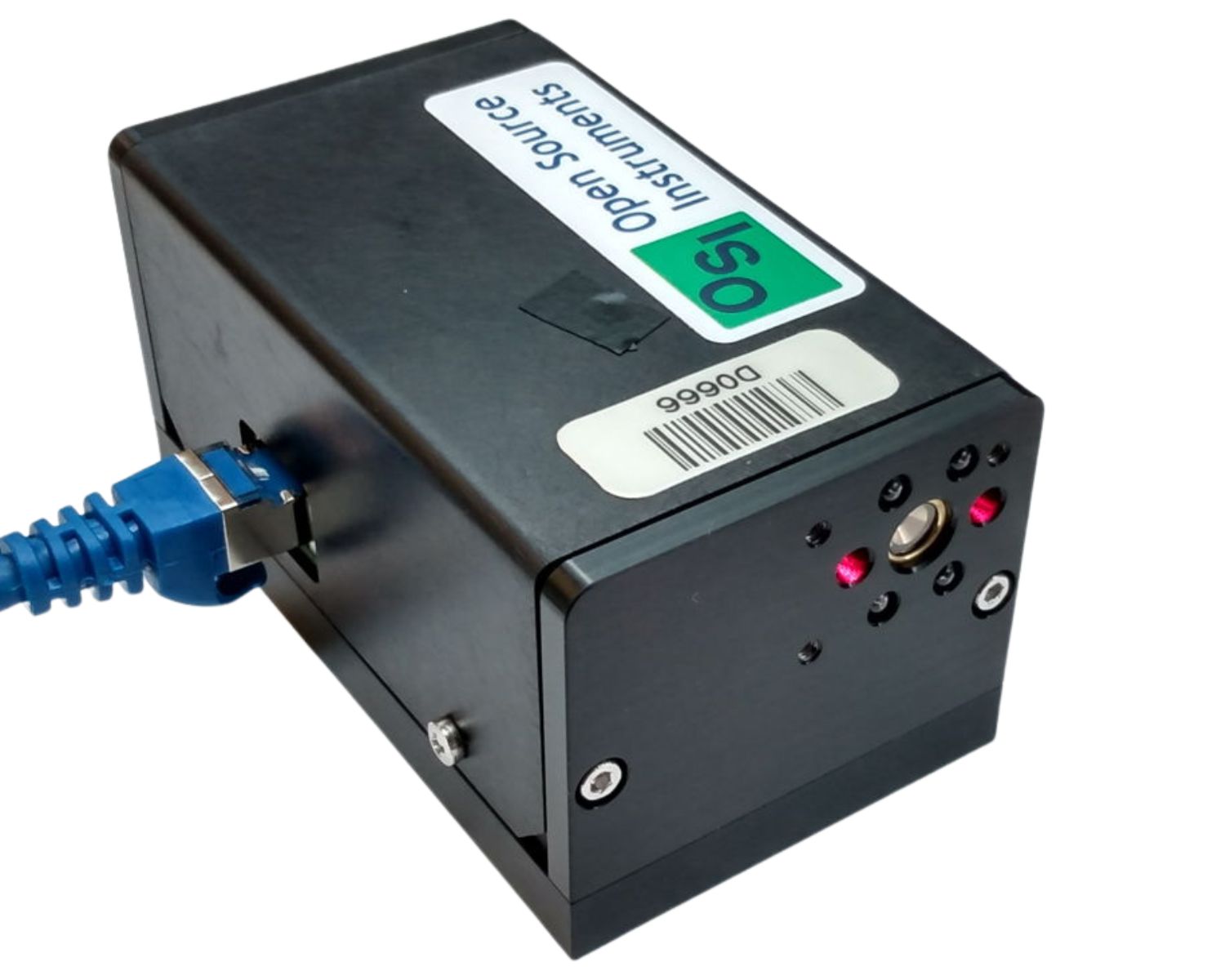
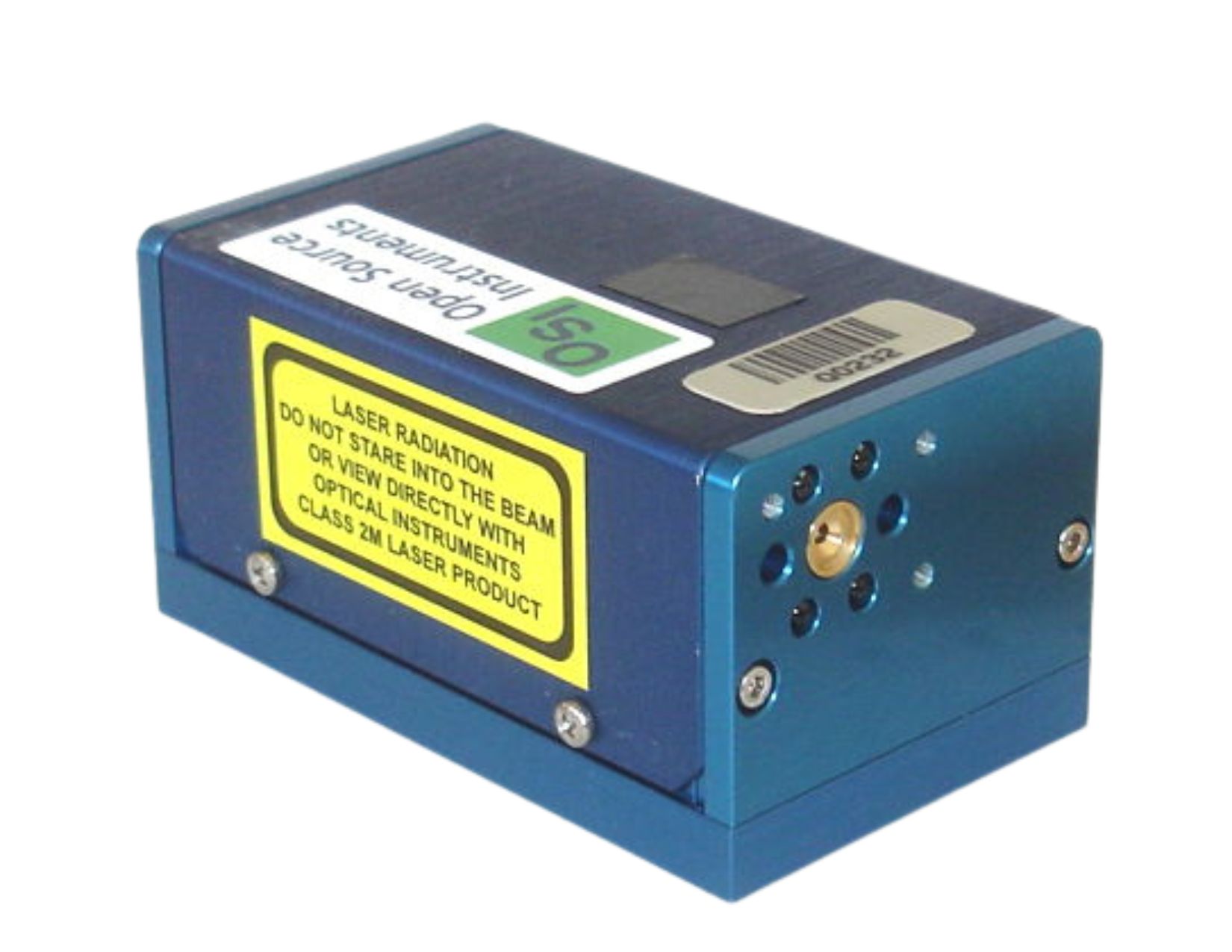