Resistive Sensor Head (A2053) Manual

Contents

Description

The Resistive Sensor Head (A2053) is a Long-Wire Data Acquisition (LWDAQ) Device that measures the resistance of up to eleven resistive sensors. These sensors could be 1000-Ω RTDs (resistance-temperature devices), 100-Ω RTDs, 120-Ω strain guages, or any similar resistive sensor. You can use the A2053 with the Guage, Thermometer, or Flowmeter. For examples of the A2053 in action, see the Examples section.

Figure 2: RTD Head (A2053A) with Enclosure. Connectors 1 through 4 are marked in numberals the box itself. Pin 1 of each connector is at the left end. Connector 4, for RTD 11, is left open in the A2053A. The resistive sensor channel numbers are marked in black numerals around the outside of the box.

The RTD Head (A2053A), for example, connects to 1000-Ω RTDs and measures their resistance with 0.1-Ω precision over the range 860 Ω to 1160 Ω. With the help of a calibration program we can use the A2053A to calibrate 1000-Ω RTDs with 0.1°C accuracy. The Strain Guage Head (A2053S) connects to up to eleven 120-Ω strain guages and measures their resistance with precision 0.01 Ω over the range 110 Ω to 130 Ω.

The A2053 connects to each of its sensors with a twisted pair of insulated, stranded copper wires. The resistance of these wires adds to the resistance of the sensor. If the sensor is a 1000-Ω RTD, a 10-m cable made out of twisted pairs pulled from a CAT-5 cable adds a constant +0.5 °C offset to the apparant temperature of the resistor. The resistance of the wires is roughly 1 Ω per 10 m. Because the resistance of such wires does not vary significantly with temperature, a one-point calibration of each sensor is sufficient to remove the effect of the wires.

Instead of running current continuously through the sensors, or using a Wheatstone Bridge to compensate for various electrical and thermal errors, the A2053 runs a small current through the sensor for a few tens of milliseconds. Because the A2053 is connected to a LWDAQ, we can digitize this voltage, display it on the screen, and take its average value. Once we have obtained this average value, we instruct the A2053 to run the same current through the bottom reference resistor on its circuit. With our 1000-Ω RTDs, we use a 1060-Ω resistor, which corresponds to a perfect 1000-Ω RTD at 15.38 °C. We record the voltage again, then select the top reference resistor. For the 1000-Ω RTDs, this resistor is 1100 Ω, corresponding to 25.69 °C. We now interpolate between the top and bottom references to obtain the resistance of the sensor.

In other words: the accuracy of the A2053 is contained in its precision resistors. Precision resistors are stable and inexpensive. They are small, rugged, and we can put them right next to our measurement circuits. The absolute accuracy of our RTD Head (A2053) is better than 50 mK, which is far less than the accuracy of the sensors we use.

In addition to resistance measurement, all versions of the A2053 provide a 15-V heating connection to any one of the sensors. Heating the sensors allows us to measure the cool-down time constant of the sensor in, for example, a pipe with flowing gas, and thus deduce the gas flow rate. The A2053F uses the heater to measure gas flow rate, as we describe here.

The A2053 mounts to a flat metal surface with four M6 bolts. The same bolts hold the A2053 circuit board to the top face of its enclosure. The drawing below shows the locations of the mounting holes. Each hole should be M6 threaded and at least 7 mm deep. Allow at least 40 mm height for the enclosure and its electrical connections.

Figure: Mounting Holes.

All versions of the A2053 connect to their eleven sensors through two eight-way plugs, one four-way plug, and one two-way 0.1" footprint that we usually leave unloaded to allow you to put a sensor right on the circuit board. Two wires connect to each sensors. The table below gives the LWDAQ element number corresponding to each pair of sensor connector pins. For an annotated photograph, see here.

See below for instructions on preparing sensor connections to fit the plugs on the A2035.

Versions

The following versions of the A2053 exist.

The A2053A uses EL2244CS op-amps. It performs well with the LWDAQ Thermometer.

The LWDAQ Flowmeter instrument, however, takes samples from a single RTD sensor for several seconds at a time without sampling the reference channels, and is unable to keep track of the offsets that grow in its EL2244CS op-amps during the measurement. We discovered this offset problem only after we had made several hundred A2053A boards with the EL2244CS. The A2053F is identical to the A2053A, but its three EL2244CS op-amps are replaced with three OPA2277UA op-amps in the same SOP-8 package. Therefore, the A2053F can be used as a Thermometer, but the A2053A does not perform well as a Flowmeter.

The A2053S is designed for use with 120-Ω strain guages, such as the 032UW by Vishay. It is incompatible with 1000-Ω RTD, and also with 100-Ω RTDs.

Connectors

The connectors used on the A2053 (as well as other assemblies like the A2044) come from the C-Grid family made by Molex-Waldom. Do not confuse the C-Grid family with the C-Grid III family. Connectors from these two families do not mate together.

The C-Grid plugs are single-row headers with pins on a 0.1-inch pitch. Each plug is enclosed in a plastic shroud. The shroud provides a keeper for a latch on the mating socket. The table below gives the Molex-Waldom and Digi-Key part numbers for C-Grid plugs, receptacles, and crimp terminals we use in our assemblies.

We strip a couple of millimeters of insulation off each sensor wire and crimp to each wire a female terminal. There are two crimps on each terminal. One should crimp the wire and the other should crimp the wire insulation. We like to use gold-plated crimps, but if you are going to connect your sensors only once, tin-plated crimps are just as good, and less expensive.

When we have the terminals on the wires, we push the terminals into a receptacle. They lock in place. We can remove them again with the help of a pin. The receptacle itself can provide a locking latch and polarization, or it can be without polarization and without the locking latch. When you have plenty of space to grab the connectors when you want to remove them, we recommend the locking receptacles. But when there is little space for your fingers, you can use the receptacle without the latch. The disadvantate of the connector without a latch is that it does not provide polarization either, so you can plug it in the wrong way around. You must look at the triangle in the receptacle face and match this up with pin one on the plug.

When we crimp our terminals, we like to use the manufacturer's crimp tool (part number 11-01-0209). But we can also get the job done with a pair of needle-nosed pliers and a little more time and effort.

Sensors

With adjustments to its reference resistors, the A2053 can be used with any resistive sensor. We obtain best performance with sensors of resistance between 100 Ω and 1M Ω where the resistance of the sensor varies by only ±10% over the measurement range.

A 1000-Ω RTD has nominal resistance 1 kΩ at 0 C. Its resistance increases by approximately 4 Ω/C. The combined resistance of the wires leading to a sensor adds to the resistance of the sensor itself, causing an increase in measured temperature of 0.25 C/Ω.

Example: We observed a 50 mK/m increase in measured temperature with our standard stranded-core twisted pair cables. The longest connection to an RTD in ATLAS is nearly five meters, which introduces an increase in absolute temperature measurement of 0.25 C. But the ATLAS temperature sensors will be calibrated a 20 C, thus removing any absolute error in the error in the absolute temperature measurement, either due to cable resistance or the sensor itself. Our ATLAS temperature sensors are accurate to ±0.3 C at 0 C, so the error due to connecting wire resistance is comparable to the error due to the sensor itself. Furthermore, if we know the length of the cable, we can calculate and remove the effect of its resistance.

The effect of the wires will be ten times greater for 100-Ω RTDs. That's why we prefer 1000-Ω RTDs for use with the A2053.

The dominant application of the A2053 so far has been the A2053A with 1000-Ω RTDs in ceramic packages with radial steel wires. In 2004, we bought five hundred RTDs with 300-mm teflon-insulated leads from Enercorp for $5 each. We installed these in the ATLAS detector. In 2008 we bought one hundred RTDs with short, tin-plated steel leads for $2 each. Most RTD leads are steel, and so must be tinned with the help of acid flux before solderin. (See solder joints for details of soldering steel wires.) Another source of radial-wire RTDs is Omega Engineering, which sells radial-lead 100-Ω RTDs for $1 each in packages of 100, or 1000-Ω RTDs for $1.50 each. At Digi-Key you will find surface-mount 1000-Ω RTDs and radial-wire 100-Ω RTDs.

Specification

The A2053 complies with the Long-Wire DAQ specification. It supports no device-dependent LWDAQ jobs. It has no Device Type and no Elment Numbers.

To determine the command word that will implement a particular operation on the A2053, write out sixteen bits in a row, starting with bit sixteen (DC16) on the left, and ending with bit one (DC1) on the right. Set each bit to zero or one as you require. The left-most four bits form the most significant nibble of the sixteen-bit command word. The right-most four bits are the least significant nibble. Translate each nibble into a hex digit, and you have the hex version of the command word.

The T1 through T11 bits select Sensor 1 through 11. The HEAT bit applies 15 V to the selected sensor or sensors, heating one or all of them. Each heated sensor consumes 15 mA from the +15 V supply, and receives 200 mW of heating power. The WAKE bit wakes up the board by turning on the ±15 V supplies. The TB and TT bits select the bottom temperature reference resistor and the top temperature reference resistor respectively. The LB bit enables the logic loop-back driver, and is used by a LWDAQ Driver's loop job.

Example: To select the top temperature reference, we set the following bits: TT (DC6) and WAKE (DC8). All other bits should be cleared. We compose the following binary number: 0000 0000 1010 0000, which translates to 0x00A0 (our symbol for hexadecimal numbers is "0x"). To heat the same sensor we transmit 0x02A0.

Example: The RTD Calibrator program reads all ten inputs and allows us to calibrate 1000-Ω RTDs with 0.1°C accuracy.

The A2053 does not respond correctly to the loop job. The loop time we measure with an A2053 is always 0 ns because the A2053 drives R LO when we send it the command that usually sets up a device for loop-back of T.

Measurement

You will find the schematic of the Sensor readout circuit here. The schematic gives the component values for the A2053A, which reads 1000-Ω RTDs. Resistor R25 sets the current flowing down out of U16-1 (the collector of the current source transistor), along K+ (the current does not go into Q18, because Q18 is the heater, and we assume it's turned off), and so to all the sensors via the common K+ connection. But the current flows through only the one sensor whose selection switch (these are the mosfets Q5..Q17) is turned on. The voltage on K+ is the voltage developed across the selected sensor when the measurement current flows through it. When R25 is 2 kΩ, the current is 350 μA. Across a 1000-Ω resistor, this current develops a voltage of 350 mV.

Figure 1: RTD Head (A2053A) Circuit Board, Top and Bottom. The RTD connectors are 0.1" shrouded headers. R23 is the center reference resistor. R26 is the top reference resistor. R27 is the bottom reference resistor. R24 sets the current through the center reference resistance. R25 sets the current through the measurement resistance, which can be R26, R27, or a resistor connected to one of the eleven sensor inputs. Normal operation of the A2053 requires that R24 and R25 be matched to 0.1%.

Resistor R24 sets the current flowing into the center reference resistor, which is R23. We make R24 close to R25, so that the sensor current and the center reference current are the same. That's why the schematic specifies R25 and R25 to 1%. (If you use 5% resistors from the same reel, they almost always agree to 1%. But we used 1% 2 kΩ resistors from the same reel in our mass-produced A2053As.) The center reference resistor has the resistance we expect of our sensors in the center of our desired dynamic range. In the case of the A2035A, we want to measure temperatures close to 20 °C in an experiment hall with 1000-Ω RTDs. These RTSs have resistance 1000 Ω at 0 °C, and their resistance increases by roughly 4 Ω/°C above that. So the A2053A center reference is 1080 Ω.

The two voltages K+ and K− proceed to the input of a differential amplifier shown here. The amplifier consists of two op-amps in package U15. It amplifies the difference between K+ and K−, which we call K, and sends the amplified difference back to the LWDAQ driver for low-pass filtering at 10 kHz followed by sixteen-bit digitization.

The useful voltage range of K is around ±40 mV. When the sensor resistance equals center reference resistor, K will be zero. With a reference current of 350 μA, K will be +40 mV when the sensor resistance is ≈110 Ω higher than the center resistance. Likewise, K will be −40 mV when the sensor is ≈110 Ω lower. The 350-μA reference current gives us a dynamic range of ±110 Ω. With 1000-Ω RTDs, this ±110 Ω gives us a dynamic range of ±28 °C, which is why the A2053A operates over a 55 °C range.

The accuracy of the A2053 comes from its use of two reference resistors. These are R26 and R27 in the schematic. The A2053 treats these just like sensors. But they are not sensors, they are known resistance values to which we compare the sensors. Resistor R27 is the bottom reference resistor and R26 is the top reference resistor. In the A2053A these are 1060 Ω and 1100 Ω respectively, and both are accurate to 0.01%. They are model SM5 wire-wound resistors from Reidon. They represent 1000-Ω RTD temperatures 15.38±0.03 °C and 25.69±0.03 °C respectively.

To measure the resistance of a sensor, we select the bottom reference resistor, then the sensor, then the top reference resistor, and we measure K for each. We interpolate between these values of K, and our known reference resistances, to obtain the sensor resistance. We then convert the sensor resistance into temperature or strain using the sensor manufacturer's data sheet.

A2053A

These component values in the schematic give the A2053A the following properties.

• Compatible RTD: 1000-Ω at 0°C, temperature coefficient 3850 ppm/°C.
• Measurement Current: 300 μA.
• Dynamic Range: 20±35°C.
• Sensor Self-Heating: See RTD manufacturer specification.
• Sensor Accuracy: See RTD manufacturer specification.
• Precision: 20 mK.
• Accuracy: 50 mK at 20°C.
• Reference Temperatures: top 25.69±0.03°C, bottom 15.38±0.03°C.
• Reference Resistors: top 1100±0.1Ω, bottom 1060±0.1Ω.
• Range Resistors (R24 and R25): 2.0 kΩ.

In other words: the A2053A measures resistance to 0.1 Ω precision over a dynamic range of 860 Ω to 1160 Ω, which is 300 ppm of the dynamic range. With the help of a calibration program we can use the A2053A to calibrate 1000-Ω RTDs with 0.1°C accuracy.

A2053E

The A2053E has R24 and R25 set to 5.6 KΩ instead of the 2 kΩ we use in the A2053A. The dynamic range of the thermometer with 1000-Ω RTD sensors is −50 to +115°C, which covers the natural temperatures we are likely to encounter in Boston, as well as the boiling of water.

A2053F

The A2053F is identical to the A2053A, except that it uses precision op-amps, the OPA2277 instead of the EL2244CS. The precision op-amps avoid offset drifts during the prolonged measurement period of the Flowmeter.

A2053S

The A2053S operates with 120-Ω strain guages like the 032UW. We want the center of our dynamic range in strain to be 0% strain, so our center resistance, R23, must be 120 Ω. The sensor's guage factor is around 2.0, so its resitance increases by 2% for each 1% strain (length increases by 1%), or 2.4 Ω for each 1% strain. To give the A2053S a ±4% dynamic range, we need to measure resistance between 110 Ω and 130 Ω. With a measurement current of 4 mA, the dynamic range of the A2053S would be 110−130 Ω. But we find that a measurement current of 4 mA gives poor performance. The measurement current source transistors heat up, and perform less well as constant-current sources. We find this is the case for measurement currents greater than 1 mA. So we use 1 kΩ resistors for R24 and R25, and set the measurement current to around 700 μA.

Now we pick the top and bottom reference resistors. Let them be 125 Ω and 115 Ω, wire-wound 0.01%, < 10 ppm/°C temperature coefficient. These values correspond to at +2.08±0.005% and −2.08±0.005% strain respectively.

These component values give the A2035S the following properties.

• Compatible Strain Guage: 120-Ω at 0% strain, 2.0 guage factor.
• Compatible RTD: 100-Ω at 0°C, temperature coefficient 3850 ppm/°C.
• Measurement Current: 700 μA.
• Dynamic Range: 60 to 180 Ω, ±100% strain, −100 to +300 °C.
• Sensor Self-Heating: See manufacturer specification.
• Sensor Accuracy: See manufacturer specification.
• Precision: 10 mΩ, 40 ppm strain, 25 mK.
• Accuracy: 100 mΩ at 120 Ω, 400 ppm at 0% strain, 0.5°C at 20°C.
• Reference Temperatures: top 64.94±0.03°C, bottom 38.96±0.03°C.
• Reference Strains: top +2.08% strain, bottom −2.08% strain.
• Reference Resistors: top 125±0.01Ω, bottom 115±0.01Ω.
• Range Resistors (R24 and R25): 1.0 kΩ.

The measurement precision should be (we have yet to test one with actual stress and strain) 300 ppm of its ±4% dynamic range, or 30 ppm strain. Its absolute accuracy (ignoring the sensor's own absolute strain error) should be 50 ppm. If you want to measure strain and temperature at the same time, you can adapt 100-Ω strain guages for the 120-Ω readout with the help of a series resistor. We describe how such a combined system might work in an e-mail.

A2053L

The A2053L is for use at cryogenic temperatures (L is for Low). We calibrate the A2053L with boiling nitrogen, which is at −195.8°C, and subliming carbon dioxide, which is at -78.5°C. We use 1000-Ω platinum RTDs, just as we would with the A2053A. We bought ours from Enercorp, and they came with teflon-insulated leads soldered to the steel wires of the RTD elements. Because we do not require more than a few degrees accuracy from the A2053L, we don't bother with 0.01% reference resistors. We obtained our reference values by immersing a selection of 1000-Ω RTDs in liquid nitrogen (−196°C) and squeezing them between blocks of dry ice (−78°C, see here for squeezing).

• Compatible RTD: 1000-Ω at 0°C, temperature coefficient 3850 ppm/°C.
• Measurement Current: 38.9 μA.
• Dynamic Range: −50±150°C.
• Sensor Self-Heating: See RTD manufacturer specification.
• Sensor Accuracy: ±5°C −196°C.
• Precision: 0.5°C at −196°C
• Accuracy: ±5°C at −196°C.
• Reference Temperatures: top −78°C, bottom −196°C.
• Reference Resistors: top 700 Ω, bottom 200Ω.
• Range Resistors (R24 and R25): 18 kΩ.

To obtain the above characteristics, we set R24 and R25 to 18 kΩ, R26 (top reference) to 700Ω, R27 (bottom reference) to 200Ω, and R23 (center reference) to 400 Ω. We used the A2053L in the tests we describe here. Because of our calibration process, in which we measure the resistance of a reference RTD at the temperature of boiling liquid nitrogen and subliming dry ice, we expect the A2053L to be exact at −196°C and −78°C with our reference RTD. When we tried out other RTDs, we found that they agreed to within ±1°C at both temperatures.

Operation

We read out the RTD Head (A2053A) with the LWDAQ software's Thermometer Instrument. Here we tell you how the hardware behind the thermometer works.

To read out the temperature sensors, you transmit command words one at a time to the A2053 using your LWDAQ Driver's command job. The A2053 has a current source which you can, by sending the correct command word, direct through one of six resistors. Two of the resistors reside on the A2053 board itself, and are 0.01% precision wire-wound resistors of 1060 Ω and 1100 . The 1060 Ω resistor provides a low-temperature reference point of 15.38°C for standard 1000-Ω RTDs, and the 1100 Ω resistor provides a high-temperature reference point of 25.69°C.

When you select the high-temperature reference, by setting bit DC6 (TT) in the command word, the A2053 sends back an analog voltage that is a linear function of the high-temperature reference resistance. You digitize this voltage using the LWDAQ Driver. The A2037 driver, for example, provides a sixteen-bit ADC which will do the job with sufficient accuracy to obtain 20 mK resolution. When you set bit DC16 (BT), you obtain a voltage from the A2053 that is the same linear function of the low-temperature resistance. Now you can select the four RTDs in turn, and interpolate between the top and bottom reference voltages to obtain the temperature of the RTD.

Example: We have a RTD Head (A2053) connected to an LWDAQ Driver (A2037). We connect a single platinum temperature sensor to the first two pins of P1 on the A2053. We use the A2037 command job to send command 0x00A0 (hexadecimal) to the A2053. This command wakes up the board and selects the top reference temperature. We allow 1 ms for the A2037's 10 kHz input filter to settle. We execute an adc16 job and retrieve the sixteen-bit result. For an A2053A this will be between 29,000 and 31,000. We send command 0x8080 to the A2053, which selects the bottom reference temperature. We wait 1 ms, and execute another adc16 job. The result should be between 38,000 and 41,000. We select our temperature sensor, which is T1, with command 0x0880, wait 1 ms, and execute an adc16 job. The result should be between 0 and 65,500 provided the sensor temperature is between -15°C and +55°C. We know that the top temperature reference is 25.69°C, and the bottom is 15.38°C, so we interpolate between the two to obtain the temperature of our sensor. We are assuming, of course, that the sensor is a 1000-Ω RTD. Note that the high-temperature reference voltage at the A2037's ADC is lower than the low-temperature reference voltage.

If you want to heat a sensor, then use the following command words, which are the same as the sensor read-out select words, but with the HEAT bit set (DC9).

We use a reference socket to test our A2053 boards. The reference socket is an 8-way socket we connect to P1. Pins 1 and 2 of the referenec socket connect to a 1060-Ω 0.01% resistor, pins 3 and 4 connect to a 1100-Ω resistor, pins 5 and 6 are connected directly together with a wire, and pins 7 and 8 are left open-circuit. The temperature we measure on T1, using the procedure given in the above examples, should be within 0.03°C of the bottom temperature reference (15.38°C). The temperature we measure on T2 should be equally close to the top temperature reference (25.69°C). From T3 we get the low-temperature end of the A2053's dynamic range. For an A2053B this should be below -10°C, allowing you to use an ice-water bath to calibrate your temperature sensors. From T4 we get the high-temperature end of the dynamic range. For an A2053B this should be above 50°C, allowing you to measure ambient temperature in most electronic equipment.

The A2053 is asleep when it powers up. It also goes to sleep when you execute a LWDAQ sleep job. To measure the propagation delay of signals travelling from the driver to the A2053 and back again, you execute a LWDAQ loop job and read the loop time out of the driver.

You will find the data acquisition steps required to control and read out voltages from all versions of the A2053 in Gauge.tcl, which is the TclTk script that defines the Gauge Instrument in our LWDAQ Software. You can also look at Thermometer.tcl, which defines the Thermometer Instrument. In Driver.tcl you will find the routines that compose TCPIP messages to communicate with a LWDAQ Driver.

Flowmeter

We describe the Flowmeter instrument in the Flowmeter section of the LWDAQ Manual. You will find details of the data acquisition process in Flowmeter.tcl. The Flowmeter measures the mass flow rate of gas in a pipe by heating up a platinum RTD and measuring how fast it cools. The RTD Head (A2053) provides a heater with which you can heat a sensor in a flow of gas. The time constant of its return to ambient temperature is, for large enough flow rates, proportional to the inverse of the mass flow rate.

The flowmeter sensor is immersed in the gas flow it is supposed to measure. The flowmeter measures the temperature of the sensor, and assumes this temperature to be the ambient temperature of the gas, to which the sensor will be cooling. The flowmeter applies +15 V to the sensor by selecting the sensor with the HEAT bit set. It waits for a second or two, and then removes the +15V. It waits for another second to allow certain initial second-order cooling effects to settle down, and then begins recording the exponential cooling of the sensor towards ambient temperature. It calculates the time constant and reports the inverse-time constant to its text window.

To convert the inverse time constant into a gas flow, you need a calibration curve for the sensor in that particular gas and in a passage of that particular cross section. You will find a study of the Flowmeter's performance here. For best performance, the Flowmeter requires the A2053F (F as in Flowmeter), which uses OPA2277UA op-amps instead of our customary EL2244CS op-amps.

Strain Guage

Below is a picture of an Strain Guage (A2053S) with a Reference Plug. The Reference Plug provides four resistances by which you can check the operation of your A2053S.

Figure: A2053S and Reference Plug. Marked are (1) 109.1±0.1Ω resistor between pins 1 and 2, (2) 0 Ω short-circuit between pins 3 and 4, (3) A 100-Ω RTD between pins 5 and 6, and (4) 120±0.1Ω resistor.

If you insert the reference plug into socket 1 on the A2053S, you will be able to refer to each resistance by the element number given in the figure above. Set ref_bottom to 115 Ω and ref_top to 125 Ω to measure each reference resistor in Ohms. The short circuit allows you to see the low end of the A2053S dynamic range. If you read an empty channel on the A2053S, you will get the top of the dynamic range. The 109.1 Ω resistor corresponds to a perfect 100-Ω RTD at 23.6°C. The 120 Ω resistor corresponds to 0% strain on a perfect 120-Ω strain guage. We provide the RTD so you can test the A2053S temperature measurement. Enter 38.96 for ref_bottom and 64.94 for ref_top, and channel 3 will act as a thermometer.

Glue

When we use RTDs to measure the temperature of a piece of metal, we glue it to the metal in two stages. First we secure the sensor to the metal with cyanoacrylate (super-glue), then we cover the sensor with non-conductive epoxy. The sensor has two sides to it, one of which has a lump that secures the sensor leads to the platinum film. It is the flat side that you must glue to the metal, because the flat side is a non-conducting ceramic surface. The platinum film is on the other side, and must be kept away from any conducting surface.

Paul Mocket of the University of Washington describes the effect of glue upon the temperature measured by the sensors here. We have never noticed any effect of glue upon the sensors, but we have never measured the temperature before and after gluing in a reliable way. Some RTD users found that they had problems when they glued the wrong side of the sensor down to the metal surface. We are not surprized, because in this case the platinum film itself is in contact with the metal.

Power Consumption

We picked an A2053A at random and measured its power consumption both asleep and awake, as shown in the following table.

The A2053 consumes additional power when you neglect to select one of its reference resistors or connected RTDs. When no sensor is selected, the returned analog voltage saturates, and the A2053 op-amps drive thirty milliamps into the 100-Ω load at the end of the cable on the multiplexer or driver to which the A2053 is connected. To obtain the lower, designed, waking power consumption, we selected the top reference resistor.

Radiation Tolerance

All the components used by the A2053 are also used by the Bar Head (A2044). For a discussion of the A2044's radiation tolerance, see here. Unlike the A2044, the A2053 does not use the INA155 instrumentation amplifier, but rather builds its own instrumentation amplifier out of two op-amps and some precision resistors. The resulting circuit is as resistant to radiation as our rad-hard EL2244CS op-amp. The sensor selection we perform with NDS355AN mosfets. We discuss the radiation tolerance of these devices here.

Electronics

Here are the six pages of the A2053 circuit diagram.

You will find printed circuit board files here.

Examples

Here we give some examples of experiments we have performed with the help of the A2053. In most cases, you will find our measurements in our Excel Spreadsheet, A2053.xls.

Cocktail Ice

We discuss with our friend Eben Klemm the manner in which ice cools a cocktail. We claimed that the melting point of ice depends upon the alcohol content of the fluid it's floating in. To measure the temperature of an alcohol-ice mixture, we need water-proof temperature sensors and an A2053 with dynamic range well below 0°C. The A2035A provides −15°C to +55°C. We used an A2053E in which R24 and R25 are 5.6 KΩ instead of 2 kΩ, so that the dynamic range of the thermometer with our 1000-Ω RTD sensors is −50 to +115°C.

We put two RTDs in the fingers of a latex glove and immersed them in a beaker of ice with water. We recorded temperature, and found that both sensors settled to 0±0.05°C. We poured out the water and replaced it with pure ethanol. We agitated the mixture and recorded temperature. We continuted to agitate the mixture at random times over the next half an hour.

We use the Acquisifier Tool with this script to record temperature from the two sensors inside the beaker, and another sensor outside the beaker, at intervals. We present the temperature of the mixture in the graph below.

Figure: Temperature with Time in Alcohol and Ice Mixture.

As you can see, the arrival of the alcohol results in a water-alcohol mixture that is well below freezing. The temperature of the mixture appears to reach equilibrium for several minutes at around −8°C. We know the ice we started with as at 0°C and the alcohol was at room temperature. And yet the mixture is colder.

Cooling Water

In the ATLAS cavern, 100 m below the ground, just inside the End Cap Cryostat, in the inner radius of the innermost ring of end-cap chambers are the disks of CSC (Cathode Strip Chambers) detectors. These generate enough heat that they must be cooled by water. There are eight A2053As on each of two disks of chambers. Each A2053A has six PT1000 RTDs attached to sockets 1−3 and 5−7. Each set of eight A2053As is connected to a single A2036A multiplexer, which in turn connects through a 100-m cable to a LWDAQ Driver in the USA15 service cavern. We received reports and evidence of mal-functioning in one of the multiplexers, so we descended into the pit and recorded the temperatures for an hour and a half. During this time, the CSC group turned on the chambers and the water cooling, then turned it off. We obtained the following graph of the temperatures from element 2 on each of the eight multiplexer sockets.

Figure: Temperature of Cooling Water in CSC System.

We saw no evidence of any data acquisition problems, with the exception of one bad point at time 2480 s on multiplexer channel 3, element 2, for which the temperature jumped down to 11°C for one sample. No doubt the problems observed with this system will arise again as soon as we leave CERN, but for now we see the thermometers working well.

Circuit Warmup

Sometimes, an electronic circuit will work when it's warm but not when it's cold. Or it might work when it's cold and not when it's warm. When the board warms up, it bends away from its heat sources. Surface-mount parts on the same side as the heat source will be stretched. Those on the other side will be squeezed. If a part is cracked, the crack closes when the part is squeezed and opens when it is stretched. If it's on the same side as the heat sources, the part may work when the board is cold, but not when the board is hot. If it's on the other side, the converse may be true.

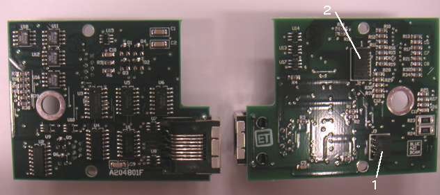
We used an A2053E to measure the warm-up and cool-down of an Azimuthal BCAM Head (A2048) as part of our investigation of two BCAMs that worked when warm but not when cold. This board has four dual op-amps that dissipate a total of 1W when the board is awake. We can see these op-amps in the SOP-8 packages on the top-left of the top side.

We attached one 1000-Ω RTD to U12 and another to the bottom side of the circuit board, opposite U12. We held the RTDs in place with a wooden clothes pin. We recorded temperature for a minute or two, woke up the board, waited for a few minutes, and put it to sleep again. We use the Acquisifier Tool with this script to record temperature from the two sensors.

Figure: Warmup of Azimuthal BCAM Head.

When the circuit is awake, the top-side (with the op-amps) is 5°C warmer than the bottom side (with the resistors and capacitors). The warm-up and cool-down are dominated by a time constant of roughly a hundred seconds.

Steel Leads

Teflon-insulated steel leads will allow us to use our RTD sensors at higher temperature, and also in smaller spaces, than our existing plastic-insulated copper wires. The disadvantage of thin steel leads is their higher resistance, which adds a significant offset to their temperature measurements, and the difficulty soldering steel wires.

We attached an RT1000 sensor to 125-μm 316 stainless steel, teflon-insulated leads. We tinned the steel leads by stripping 5 mm, coiling the exposed steel with tweezers, dipping in water-soluable acid flux, and covering with solder, as described here. We coil the sensor leads also, and tin them in the same way. We solder the tinned ends together and cover with black heat shrink to create the sensor with high-temperature, insulated, flexible leads, as shown below.

Figure: RT1000 Sensor with Stainless Steel Leads. At the end of the leads is a two-pin plug.

We measured the resistance of this stainless steel wire to be 60 Ω/m. The leads of the sensor shown above are 150 mm long, and so each has a resistance of 9 Ω. Together they present the RTD Head with an additional resistance of 18 Ω. The 1000-Ω RTD resistance increases by 4 Ω/K. In theory, the steel leads will add 4.5°C to the temperature recorded by the sensor.

We calibrated the steel lead sensor and two others by taping them to an aluminum plate and measuring the plate temperature with a mercury thermometer.

Figure: Calibration of Sensor with Steel Leads. Measurements taken with RTD Head (A2053A) at 18.8°C.

The first two sensors have copper wires of roughly 1 m, with resistance 0.2 Ω/m. The steel sensor has offset 4.8 °C, which compares well to our expected 4.5 °C.

Water-Proof

We made a water-proof sensor by starting with a sensor with steel leads and placing two silicone tubes over teflon-insulated steel wires. We coated the tubes and the sensor with silicone dispersion. We applied two more coats of dispersion to the sensor and exposed steel leads. The result is shown below.

Figure: Water-Proof RT1000 Sensor.

Sensors like this are rugged and water-proof. They can withstand temperatures of at least 200°C. The 150-mm steel leads give it an offset of approximately 4.5°C.

Greenhouse

We used three 1000-ΩRTDs to observe how convection acts to cool down illuminated surfaces. We placed a 60-W lamp over a black-anodized aluminum plate with side walls. For a photograph of our open greenhouse, see here. We arranged three sensors upon and above the plate. One we taped to the plate with black electrical tape (the plate sensor). Another was just above the plate but in shadow cast by a piece of black electrical tape (the shade sensor). The third was in the open at a height just below the side walls of the plate (the light sensor).

Between the lamp and the plate we placed a rock salt crystal. The rock salt is held just above the plate with three metal posts. We choose rock salt instead of glass because it is transparant to both visible and infrared light. Infrared radiation from the black plate will pass out through the rock salt just as easily as visible radiation from the lamp passes in.

Note: We are pretty sure this crystal is NaCl. It tastes like salt. We can scratch off fragments with a scalpel, but we cannot scratch it with our fingernails. Fragments do not react with HCl. It is soluble in water. It cleaves at right angles. The only thing we find confusing about our sample is the pyramid on top of the crystal.

Air can pass freely across the plate and around the crystal. Thus the plate will be warmed by radiation through the rock salt, and cooled by convection of air and also by radiation from the plate itself.

We began to record temperature, waited a few minutes, and turned on the lamp. The lamp proved to be near the end of its life, becaue it turned on and off of its own accord a few times until we replaced it with a new bulb. When all three sensors reached a stable temperature, we lowered the rock salt crystal onto the plate and blocked off the open sides around the plate with black tape. We show the closed greenhouse below.

Figure: Open Greenhouse.

The graph below shows the temperature we recorded from all three sensors during the entire experiment.

Figure: Temperatures Recorded from Greenhouse. We turned on the lamp at time 720 s and lowered the crystal into the closed greenhouse position at 5400 seconds. We acquired data every 60 s.

When we turn on the light, all three sensors show ris of almost 8 °C. When we lower the rock crystal, the plate and the shaded sensor show a further rise of 3 °C, while the sensor that is just below the rock salt shows a rise of 4 °C. Despite the fact that radiation can enter and leave our closed greenhouse with the same ease as the open greenhouse, the closed greenhouse is hotter. There is no change in the ease with which heat can be conducted away through the base of the plate to the table. We conclude that the closing of the greenhouse stops heat loss by convection, and that is why the closed greenhouse is warmer than the open greenhouse.

By using rock salt as a window for our greenhouse, we show that the warming of greenhouses, which are normally made of glass, has nothing to do with the fact that glass is opaque to infrared light.

Water Evaporation

We took a brass disk and placed it on top of an up-turned petri dish. On the side of the dish we taped 1000-Ω RTD with steel leads. We placed another 1000-Ω RTD with steel leads, this one coated in silicone, in a 50-ml beaker of water. We connected both RTDs to an A2053A and began to record their temperatures. We placed a 60-W lamp 150 mm above the disk and turned it on, as shown here. The disk warmed up.

Figure: Brass Disk with Water Film on Top Surface. There are two sensors: one attached to the underside of the brass disk, and the other immersed in the water layer.

After a while, we poured some of the water on the disk, so that the surface was coated with a film of water roughly 0.5 mm deep. We moved the water-proof sensor into the hole in the middle of our disk.

Figure: Cooling of Brass by Water Film. We acquired data every 60 s. We turn on the lamp and allow the shiny, dry brass disk to warm up from 18°C to 38°C. At time 5600 s, we cover the shiny brass with water that we have warmed to 38°C. The brass cools to 29°C. At time 16,000 s the water has evaporated, leaving behind a white residue. The brass is no longer shiny. It warms up to 31°C, but does not return to its previous 38°C.

When we turn the lamp on, the disk starts warming up at 0.011°C/s. The brass disk weighs 150 g. Its heat capacity is roughly 60 J/°C (0.38 J/g°C). We conclude that the disk absorbs roughly 0.63 W of radiation from the lamp. As the disk heats up, it begins to lose heat by evaporation, radiation, and convection. Its temperature reaches a new equilibrium at 37.6°C, which is 19.1°C above the ambient temperature of 18.5°C.

When we cover the brass with 0.5 mm of water, it cools down at 0.0072 °C/s, which means it is losing 0.41 W as a result of being covered by water. It reaches a new equilibrium temperature of 29°C. Three hours after covering the brass disk, the water has evaporated. The water film was 49-mm in diameter, its area is 1900 mm². The layer was roughly 0.5 mm deep to start with, so evaporation was 0.17 mm/hr, or 0.32 ml/hr. The latent heat of evaporation for water is 2.2 kJ/g, so heat dissipated from the brass disk by evaporation is 0.20 W. This 0.20 W is less than the 0.41 W loss we observe. It may be that the initial cooling of the brass was fast beause the initial evaporation loss at 38°C was greater than the equilibrium evaporation rate at 29°C.

After the water evaporated, the brass disk was covered with a non-reflecting white film. If evaporation were responsible for the cooling of the brass, we would expect the brass temperature to rise back up to 38°C once the water was gone. But the brass rose only to 31°C. We conclude that evaporation of water is not entirely responsible for the cooling of the disk.

Oil Film

We continue our study of radiation from a brass disk covered with fluid. This time, we use sesame oil as our fluid. A 1-mm film of vegetable oil is transparant to visible light and near-transparant to infrared, but it does not evaporate and it does not conduct heat as well as brass. We are curious to see what happens when we cover our brass disk with oil.

We polish our disk at the beginning of our experiment, and confirm that its reflectance is at least 80% for visible light. We allow the disk to reach its equilibrium temperature under the lamp before we start recording temperature. The polished disk rises to 34°C, which is less than the 38°C attained by the un-polished disk in our water evaporation experiment.

The brass disk (polished on the top and tarnished on the bottom) warms in the light of our lamp. It reaches 35°C. We warm up some oil and cover the disk. The disk warms up to 38°C.

Figure: Warming of Brass Disk by Oil Film. We acquired data every 60 s.

Oil conducts heat poorly, so the brass must be warmer in order to dissipate heat by convection. The radiation of heat, meanwhile, is relatively unchanged by the presense of the oil film, which is transparant to 1-μm and 10-μm radiation.

Oil and Water

We polish our brass disk top and bottom. The bottom was previously dark with tarnish. We build a wall of tape all around the top side. We warm it up under the lamp. We cover the top with 4 mm of water. This layer is thick enough to act as an insulator in comparison to the brass beneath it. We wait while the disk cools down. We cover the water with oil and stir the mixture. The oil forms a layer on top of the water, and prevents the water from evaporating. Now we will see if the effect of water without the influence from evaporation.

Figure: Warming of Brass Disk by Water and Oil Layers. We acquired data every 60 s. There are two sensors: one attached to the underside of the brass disk, and the other immersed in the water. At 1900 s we pour the water on the disk. At 3200 s we pour the oil onto the water and stir.

With the disk covered with 4-mm of water, we see the brass disk cooling by 2°. We did not allow the disk to reach thermal equilibrium before we added the water, nor before we added the oil. We estimate the difference between the equilibrium points to 4°C. But this is still less than half the 9°C cooling we observed with a 1-mm layer in our water evaporation experiment.

The thermal conductivity of water is 0.58 W/m°C, compared to 109 W/m°C for brass. We know from our previous measurements that the brass disk receives roughly 0.63 W from the lamp, and we suspect that the main source of heat loss is by convection at the top surface of the brass. In order to transport 0.63 W of heat through 4 mm water over our 60-mm diameter disk, we need a temperature drop of roughly 2°C.

We see 5° less cooling with a 4-mm layer of water than with a 1-mm layer of water. We can account for 2°C of this difference in terms of the low conductivity of water, but we cannot explain the remaining 3°C.

When we add the oil, the disk warms up again. The disk is covered with an insulating layer of water and another of oil. The water is not evaporating. The disk warms up in order to promote convection at the oil surface.

We conclude that the initial cooling is due to evaporation, and the subsequent warming is due to insulation.

Water Film

According to Stefan's Law, a black body radiates heat at a rate given by:

P = σT⁴, where σ = 5.7 × 10⁻⁸ W/m²K⁴

The flat, central region on the top side of our brass disk has diameter 49 mm and area 1900 mm². If this region were black, it would radiate 0.80 W at 20°C.

According to Wein's Displacement Law, the peak emission wavelength for a black body, in units of power per unit interval of wavelength, is given by:

λ_max = 3/T mm/K

A 60-W incandescent bulb filament operates at roughly 3000 K, so its peak emission wavelength is around 1 μm, just outside the visible range. Our brass disk is at around 300 K and its peak emission wavelength is around 10 μm, far outside the visible range.

Figure: Normalized Radiation Spectrum with Wavelength for Lamp Filament (3000 K) and Brass Disk (300 K). These plots are in units of power per unit change in wavelength and plotted on a log scale, so they do not have the same shape as the more common power versus frequency plots. For linear wavelength scale, see here.

The absorption length of water at 1-μm is around 50 mm and at 10 μm is around 10 μm. The absorption length is the parameter L in the exponential absorption equation that relates the fraction of radiation absorbed, A, to distance, x, in the absorbing material.

A = 1 − e ^x/L

After length L, we absorb 63% and after 2L we absorb 86%. Thus water absorbs 86% of 1-μm radiation in 100 mm, and 86% of 10-μm radiation in 20 μm. Thus a 20-μm film of water is transparant to 1-μm radiation from the bulb, but black to 10-μm radiation from the disk itself. We wonder what would happen if we covered the shiny brass disk with a layer that absorbs and radiates at 10-μm, but is transparant to 1-μm radiation from the lamp. Will the disk warm up or cool down?

In order to observe radiation, we must eliminate evaporation of water. Evaporation tends to coold the disk, as we saw earlier. We can stop evaporation by covering the water film with a skin of clear plastic. We cut a circle of clear plastic 60 mm in diameter from a re-sealable bag.

Our clear plastic water-cover is transparent to visible light, but we are unsure of its behavior at the 1 μm and 10 μm wavelengths emitted by the lamp and the brass disk respectively. In our experments, we will try covering the lamp itself with a sheet of the same clear plastic, thinking that radiation that passes through the lamp cover will also pass through the water cover.

Because radiated power increases as the fourth power of the temperature, we will move our lamp closer than in our previous experiments. We will try placing the lamp 60 mm above the disk and 100 mm above the disk, as compared to the 150 mm we used in earlier experiments.

Figure: Brass Disk and Plastic Cover. The lamp is 60 mm above the center of the disk.

We begin our experiment by allowing the freshly-polished brass disk to warm up on its own, with no plastic and no water, and the bulb 60 mm away. Ambient air is 30°C beneath the lamp. We don't show the initial warming because the time constant of the entire warming is thousands of seconds. The initial warming of the disk was around 0.034°C/s, which, together with the 60-J/°C heat capacity of the disk, suggests that the lamp is delivering 2 W to the disk. The disk warms up in order to dissipate this 2 W by convection through its top surface.

Figure: Water Layer Under Plastic Cover. Note sides held in by surface tension. This layer is 1 mm, which is much thicker than the one we used in our experiment, but more visible for the benefit of the photograph.

We inject 2 ml of water under the cover to form a 100-μm water film. (The film shown in the photograph was made from 20 ml of water and is 1 mm thick.) Our plastic water cover is a 100-μm thick circle of clear polypropylene. The conductivity of polyethylene is around 0.45 W/m°C. The are of the cover that is in contact with water is roughly 1900 mm². The sheet would require a temperature drop of 0.2°C to conduct the entire 2 W the disk is receiving from the lamp.

The conductivity of water is 0.58 W/m°C. Our 100-μm film would require a temperature drop of 0.2°C to transport 2 W. We don't know how much of this 2 W passes through the water and the sheet, but we see that the disk will tend to warm up because of the insulation provided by the water and the sheet.

With a red laser beam and an optical power meter, we measured the reflectivity of the bare, polished brass surface, and found it to be greater than 80%. If we assume uniform reflectance of 80%, we expect uniform absorption and emission of 20%, as dictated by the second law of thermodynamics (see here for explanation). At 20% efficiency, our 1900 mm² circle of brass will emit 0.18 W at 30°C and 0.24 W at 50°C.

The water film acts as a good emitter of 10-μm infrared, while being transparent to 1-μm light from the lamp. The film radiates 0.91 W at 30°C and 1.18 W at 50°C. The water radiates 0.27 W more at 50°C, while the brass radiates only 0.06 W more at 40°C. At 50°C, the brass-water system will lose 0.21 W more heat by radiation than the brass-only system.

We don't kow how the clear plastic cover behaves in our lamp-light, nor how it radiates its own heat. In this first experiment, the lamp light is not filtered by its own sheet of clear plastic, so the plastic cover may be absorbing near infra-red and warming up on its own.

If we ignore the plastic cover, we see that the disk will tend to cool down because the water radiates the brass's heat better than does the brass alone, while at the same time the water absorbs no heat from the lamp.

Figure: Water Film with and without Plastic Sheet. (1) Bare brass disk under lamp. (2) Add plastic cover with 100-μm water film. (3) Remove water, dry, replace plastic cover. (4) Remove plastic covert and place large plastic sheet in front of lamp. (5) Add plastic cover to disk again. (6) Remove sheet in front of lamp.

The plastic cover appears to heat up the brass plate. The water has no significant effect. Covering the lamp has a significant effect. We start again, this time with the lamp light filtered by a clear plastic sheet, and the bulb 100 mm from the disk instead of 60 mm, so that we can get our hands into the space above the lamp without moving anything. We also introduce a kitchen cling-film into the experiment. According to our calipers, this clear plastic film is only 10μm thick. The graph below shows our results.

Figure: Water Films and Plastic Sheets. The lamp is 100 mm from the brass disk and covered by a plastic sheet taped over the entire lampshade. (1) Brass disk with clear 100-μm plastic sheet. (2) Inject 500-&u;m layer of water under sheet. (3) Neon lights go off in lab while we are out. (4) Neon lights go on again when we return. (5) Remove disk cover and dry off the disk. (6) Remove lamp cover. (7) Cover disk with 100-μm plastic sheet again. (8) Replace 100-μm plastic cover with circle of 10-μm cling-film. (9) Inject 500-μm layer of water under cling-film. (10) Suck out water to reduce water film thickness to 100 μm. (11) Temperature appears stable, so end experiment.

Here is a table of the equilibrium temperatures.

If you work your way through all these steps, you'll see that a 500-μm water layer warms up the plate, but a 100-μ layer cools it down. When we reduce the water layer from 500-μm to 100-μm the disk cools by 2.8°C. The 100-μm water film cools the disk by 1.7°C compared to no water film.

The thicker layer of water acts as an insulator with respect to heat leaving the brass by convection at the top surface. Therefore, it causes the disk to warm up. The thinner layer conducts heat well, but still radiates as effectively as the thicker layer. The disk starts to cool down.

The cooling caused by the thin layer does not proceed according to a first-order exponential step. The change does not appear to have a time constant. Such behavior suggests some kind of feedback in our cooling system, and indeed, there is a clear source of feedback. Most of the 1 W the disk absorbs from the lamp is leaving through the top surface by convection. When the water cools down the top surface, the convection slows, which means the top surface must heat up again to promote the heat flow. We predict that we will see first-order exponential cooling with a water film beneath the disk.

Cling-Film Diaper

Following our water film experiment, we would like to isolate cooling by radiation from cooling by evaporation, conduction, and convection. We would like to accelerate the cooling also, so that we can observe the effect more easily. Instead of covering the top surface of our brass disk with water, we cover the bottom surface with the help of a diaper made of kitchen cling-film.

Figure: Cling-Film Diaper around the Brass Disk. Note that we now place the brass sensor on the top surface. The cling-film is taped with black electrical tape.

We allow the plate to warm up beneath a 60-W bulb. The bulb is 100 mm above the top surface. The initial slope of the warm-up is 0.030 °C/s, which implies heat from the lamp to the surface of 1.8 W.

Once the disk reaches equilibrium, we realize that we must raise it up off the petri dish to allow water to collect in the cling-film diaper. So we raise the disk with two washers and wait a while longer for a new equilibrium.

We inject hot water into the diaper through the tape-covered hole in the center of the disk, from above. We are not sure how thick the water covering of the disk is. The thickness varies. But our best guess is 500 μm average thickness. We replace the disk and wait.

Figure: Water Cooling Brass Disk by Radiation. The lamp is 100 mm from the disk. The disk sensor is on the top surface. (1) Brass disk with cling-film diaper, no water. (2) Raise disk on two washers to allow space for water in diaper later. (3) Inject hot water into diaper through central hole in top surface of disk. We repeated the experiment a week later and obtained this plot, which shows a 2°C drop after injection.

We should have waited longer after we raised the disk, to allow the disk to return to its equilibrium temperature of 49.4°C, but we were too hasty. We assume, however, that the disk would have returned to this same equilibrium had we given it the opportunity to do so, or perhaps a slightly higher equilibrium, now that it is 1 mm closer to the lamp as a result of the thickness of the waters.

We get a 2.4°C drop in the equilibrium temperature as a result of adding a layer of water to the bottom surface. We see a jump downwards when we inject the water, but that's because the water was not as hot as the disk. After that, we see a first-order exponential approach to a new equilibrium temperature.

Our ambient temperature is 26°C. The disk will radiate heat at wavelengths around 10 μm. Water is black to these wavelengths, and therefore a 100% efficient emitter. Our polished brass is 80% reflecting, and therefore a 20% efficient emitter. The bottom surface of the disk has area roughly 2000 mm². At 26°C it will radiate 0.91 W when covered with water and 0.18 W as bare brass (for physical laws and constants see above). At 47°C, the water will radiate 1.19 W and the brass will radiate 0.23 W. Thus the water-covered surface radiates 0.28 W more at 47°C and the bare brass surface radiates 0.05 W more. By switching from brass to water, the disk will radiate 0.23 W more heat. That's why it cools down.

Given that the total heat absorbed by the disk from the lamp is roughly 1.8 W, this 0.23 W additional radiation causes a 13% drop in the heat flow by convection out the top surface of the disk. To the first approximation, therefore, we expect a 13% drop in the temperature above ambient that we measure on the top surface. Without the water, the top surface is at 49°C, which is 23°C above ambient. So we expect a 3°C drop when we add water. What we see is a 2.4°C drop. That's close enough for our liking.