
Figure: Image from ICX424 During Irradiation, Accumulated Dose 140 Gy. No image intensification. Exposure time is 50 ms. The black circle is the shadow of a 2.5-mm tungsten ball.
| DEC-13 |
| MAR-14 | APR-14 | AUG-14 | OCT-14 | |
| NOV-14 | DEC-14 |
| JAN-15 | FEB-15 | MAR-15 | APR-15 | |
| MAY-15 | JUN-15 | JUL-15 | NOV-15 |
| FEB-16 | MAR-16 | APR-16 | MAY-16 | |
| JUN-16 | SEP-16 | NOV-16 | DEC-16 |
| JAN-17 | MAY-17 | SEP-17 |
| JAN-18 | MAR-18 | MAY-18 | JUN-18 | |
| AUG-18 | OCT-18 | NOV-18 |
| JAN-19 | FEB-19 | MAR-19 | SEP-19 |
| APR-21 |
[13-DEC-13] We place a 1.27-mm thick (0.343 g/cm2) Al absorber in front of our continuous source. The absorber eliminates almost all x-rays below 14 keV. Our x-rays are generated with a 50-keV anode voltage, so their maximum possible energy is 50 keV. For these x-rays, energy deposition per unit mass density in silicon is 7.3 times greater than in air. Furthermore, x-rays in this range are almost certain to penetrate the window of our image sensor.
We place a TC255 and an ICX424 image sensor at range 55 cm from the source point. We place a 2.5 mm diameter tungsten ball over the window of the ICX424. We place the readout electronics behind a lead brick. At the plane of the image sensors, the Radcal Dosimeter, with its 60 cc ionizing chamber, measures 1.7 R/min, which is 6.6 Gy/hr in Si. We will apply power to the image sensors only when we acquire images, which takes a fraction of a second. At all other times, the sensor heads will be asleep, and no power will be applied to the sensors.
We start our experiment at 6:15 pm on 12-DEC-13. After 22 hours we have accumulated 140 Gy. The TC255 image sensor appears to be unaffected by the dose, but the ICX424 shows clear signs of damage.
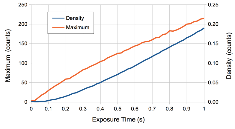
The small, bright spots in the image are x-ray hits. Every image we take has a different collection of such spots. Outside the shadow of the tungsten ball, the accumulated radiation dose has turned the image gray. The following graph shows how the average and slope of intensity vary as we accumulate a dose of 450 Gy.

There are four measurements that deviate from the trend. In previous work, we determined that these measurements correspond to white images. These white images occur at random during irradiation, but not when we stop the irradiation. In this case, there are four white images out of four hundred taken during the irradiation.
During our experiment, we use single-pixel readout of the ICX424. After exposing the image area for 100 ms (0-140 Gy) or 50 ms (140-450 Gy), we transfer all the image pixels into the sensor's transfer array. This transfer takes place in one step. The pixels in the top row are read out first. They spend less than 1 ms in the transfer array. The pixels in the bottom row spend 200 ms in the transfer array. The slope of intensity tells us how fast the pixels are filling with charge while they are in the transfer array.
After 450 Gy we stop the irradiation and obtain the following image from the irradiated sensor with a DSL821 lens, a modified HBCAM Head (A3025), and quadruple-pixel readout. We decreased the gain of the A3025's amplifier so the saturation level of the quadruple pixel readout dropped to 191 counts from >255 counts. We take hundreds of images with the lens, and see no intermittent problems with data acquisition. Nor do we see any degradation in the sharpness of the images.

We connect a temperature sensor to the image sensor glass and cool down the sensor to −25°C. We allow it to warm up in the dark with a hot aluminum plate to take its temperature above ambient. We take 100 ms exposures in the dark and obtain the following plots of average and slope of intensity in the right side of the image with quadruple-pixel readout.

The average and slope of intensity increase exponentially with temperature. When we vary the exposure time for dark images, the average intensity increases linearly with exposure time. We conclude that ionizing radiation damages the ICX424 in such a way as to increase its dark current. After 450 Gy, we can still use the sensor to take images at 20°C with exposure times up to 100 ms.
[16-DEC-13] We place another ICX424 in our continuous x-ray beam, as in our previous experiment. Every hour we capture an image from the ICX424 with quadruple-pixel readout and an image from the TC255 with single-pixel readout. This is the same TC255 that received 450 Gy in our previous experiment. Both sensors are receiving 6.6 Gy/hr.
[18-DEC-13] Our ICX424 has received 300 Gy. We take the following image with quadruple-pixel readout. We intensify with our "strong intensification" to show the radiation hits and the slope of intensity.

The graph below shows how slope and average of intensity for the ICX424Q images increases with dose so far. We take one measurement per hour.

[19-DEC-13] We stop the ICX424 irradiation at 5:00 pm today at a total dose of 475 Gy. We enter the x-ray room and turn on the continuous source again, and obtain 1.6 R/min, which is slightly less than the 1.7 R/min we have assumed in our plots. We will leave our plots as they are. We allow the sensor to take video images through a lens. We obtain this image at 20°C with 10-ms exposure time.
[18-MAR-14] We place our TC255 Dosimeter at position 70 cm on our x-ray table, which is 55 cm from the continuous x-ray source. At the same location we place three C460EZ500 LEDs mounted to LED Heads (A2079B) and connected to a Fourteen-Way Switch (A2078A) with six-way flex cables. With these circuits, we can flash the LEDs from the LWDAQ. We set up a Camera Head (A2056) to view the LEDs as they flash. Each LED appears as a spot of light in the camera image. With the BCAM Instrument, we obtain the total intensity of each spot. This total intensity will be a measure of the power emitted by the LED during our irradiation. Our Acquisifier script is RTT_2. We cover the TC255 image sensor window with two coats of black nail polish so that dim light in the x-ray room won't disturb the detection of x-rays. We place our Radcal Dosimeter at the same position, 55 cm from the continuous source. We take data for a few minutes to confirm the stability of our intensity and dosimeter measurements with no light and no x-rays. We ramp up the continuous x-ray source and obtain a steady 1.64 R/min = 6.3 Gy/hr in Si.

One hour into the experiment, we had to go in and adjust the fan, which upset the brightness measurements, because we moved the LEDs slightly and the camera too. When we get to 450 Gy and we still see no drop in LED intensity, we check the x-ray dose rate with the TC255 dosimeter as follows. We turn off the x-ray source. We take an image with the TC255. Its average intensity is 59. We turn on the x-ray source. We take another 50-ms exposure and apply a threshold of 62 to determine the charge density of the hundreds of bright x-ray hits. The charge density is 0.665 counts/pixel. We refer to this graph of charge density versus dose in Roentgen, which has slope 523 counts/px/R. The TC255 image indicates a dose rate of 1.5 R/min, which is consistent with the Radcal's 1.64 R/min. Our x-ray source is still running.
[25-MAR-14] Our three blue EZ500 LEDs have received 1000 Gy. We see no change in their brightness when supplied with current through an 86-Ω resistor from 15 V. We stich on each LED in turn and measure it forward current with the LWDAQ power supply monitors. They draw 142 mA, 142 mA, and 143 mA. We remove the LEDs from our test stand and install an un-exposed LED. It draws 143 mA. During our 1000 Gy radiation of a bare die LED, we see no change in its optical power output or forward voltage drop.
We restore our three blue LEDs, although not necessarily in the same locations. We move the Fourteen-Way Injector (A2078A) circuit to the same 70-cm location on our tape measure, perpendicular to the x-ray beam, so that all its circuits, and the TC255 dosimeter, and the LEDs receive 1.64 R/min = 6.3 Gy/hr. We use Acquisifier script RTT_3 to measure the charge density due to x-rays in the TC255 image sensor and the quiescent current of the LWDAQ circuits drawn from the +5 V power supply. The A2078 uses an LC4064ZC and an SN65LVDS180D transceiver, both of which may suffer from increased quiescent current as a result of ionizing radiation damage. The LC4064ZC is an EEPROM-based non-volatile programmable logic chip. We make sure our new script sorts the three LED images in order of increasing x rather than brightness. We turn on the x-ray source and start running. The charge density in our TC255 dosimeter is 0.67 counts/px, which implies a dose rate of around 1.5 R/min, but we will stick with the Radcal's measurement of 1.64 R/min. We will trust the TC255 dosimeter to monitor changes in dose rate, but not the absolute dose rate.
We run for a couple of hours, accumulating roughly 12 Gy in Si. The x-ray head is at 47.5°C. We stop the experiment, entere the x-ray room and re-arrange the apparatus so the fan is blowing more effectively on the x-ray head. The photograph below shows our setup. We re-start the experiment. We keep in mind that our LEDs have already endured 1000 Gy and our A2078A has endured 12 Gy.

The fan blows into the opening in our lead brick x-ray source enclosure. We like to keep the temperature of the x-ray head below 40°C. If the temperature exceeds 50°C our data acquisition script will shut down the x-ray source.

When we turn on the x-ray source, the +5V quiescent current increases by 7.7 mA. This current is drawn by the connection between the LWDAQ and the x-ray controller, and is not the result of any increase in current caused by the absorption of x-rays in the electronics. The excess current plotted above is with respect to the first moments the x-ray source is turned on.
[04-APR-14] Yesterday, our 25-MAR-14 irradiation was stopped by a power cut. Today we enter the x-ray room and place our Radcal dosimeter on the table just in front of our A2078A circuit board. The disk of our Radcal Dosimeter's 60-cc ionizing chamber covers the A2078A logic chip. We turn on the x-ray source. The dose rate is 1.70 R/min, or 6.5 Gy/hr in Si.
We start a new irradiation. We leave the TC255, A2078A, and three EZ500s in place. We add a Laboratory Camera (A2075B) with a fresh ICX424 mounted on the board with no lens. We cover the ICX424 window with two coats of black nail polish. Apparatus shown below.

We use the RTT_4 Acquisifier script to obtain the charge density and average intensity of the TC255 and the ICX424, the brightness of the LEDs, and the total inactive state current consumption of the LWDAQ devices. In the graph below we show the average intensity of the ICX424 image with a 50-ms exposure and single-pixel readout, and the excess +5V quiescent current.

The excess quiescent current starts at 3.1 mA following our earlier irradiation of the A2078A. Now our excess quiescent current arises from damage to the A2078A and the A2075B. The A2078A flashes the LEDS all the way through the experiment, and the EZ500 average intensity remains constant to ±5%. The A2075B reads out the ICX424 all the way through the experiment. The two spikes in average intensity also occurred in earlier experiments, when the A2075B was shielded behind lead.
Meanwhile, the ICX424 shows the same rate of dark current increase as in our previous irradiations. We decrease the gain of the A2075 output amplifier by changing R31 and R32 to 330 Ω. We obtain the following image with continuous 3 frame/s quadruple-pixel readout. The ICX424 draws 7 mA from 15 V during exposure and readout, which take roughly 50 ms. The average power dissipation at 3 frames per second is 16 mW. The thermal resistance of a typical DIP package is of order 100 °C/W, so we expect our ICX424 silicon to heat up by roughly 2°C. A °C rise will increase the dark current by no more than 20%. We obtain the following image with a 1-ms exposure at 3 frames/s in our laboratory at 19°C ambient temperature.

This is the third ICX424 we have irradiated with our continuous x-ray source. All show the same increase in dark current with dose.
[22-APR-14] Starting on 15-APR-14, we run our first experiment with Brandeis University's gamma-ray Irradiation Chamber. The cesium source produces 660 keV gammas rays as well as beta particles. But the beta particles are immediately absorbed by the source's shielding, so that only the 660-keV gamma rays reach our electronics. Our objective is to determine whether our measurement of the dose delivered by x-rays to silicon is correct. With 660-keV gammas, we do not have to correct for the absorption coefficient of silicon, on account of the absorption coefficients of air and silicon being the same 0.030 g/cm2 at 660 keV. When we irradiate with x-rays, we multiply the dose in air by 7.3 to obtain the dose in silicon, to account for the higher absorption coefficient of silicon compared to air.
We install the irradiation chamber's ×10 absorbers. We intend to install our electronics within the chamber at Position 3, which we measure to be 18 cm from the source. According to the Brandeis University documentation from 1986, and accounting for the half-life of Cs-137, the dose rate at Postion 3 should be 8.2 R/min, or 4.3 Gy/hr. When we place our battery-powered Radcal Dosimeter into the chamber, with the ionizing chamber at Position 3, we measure 5.7 R/min or 3.0 Gy/hr in air or silicon at Position 3. In our analysis, we will use the dose we measured with our Radcal Dosimeter because this is the same dosimeter, calibrated in September 2013, with which we calibrated our x-ray doses.

We mount two ICX424 Minimal Heads (A2076E) to the front side of a piece of cardboard and connected by 50-mm flex cables to a Blue HBCAM Head (A3025B) on the back side. Each A2076E provides one ICX424 image sensor. We paint the sensor windows with three coats of black nail polish to block ambient light. We fasten the cardboard to an aluminum block and place it inside the irradiation chamber so that the sensors are at the range of Position 3 and centered upon the height of the chamber. The A3025B is 1.5 cm farther from the radiation source. We close the chamber and raise the source into position. We set up our data acquisition system outside the chamber.

With the door closed and the source raised, we obtain the following image of gamma rays with one of the image sensors. The exposure time is 50-ms.

We take one image from each sensor each hour, record charge density and average intensity, and save both images to disk. We calculate the dose rate at We obtain the following graph of charge density and average intensity in the two image sensors versus measured ionizing dose.

The average intensity increases linearly from 0-400 Gy. The slope is 0.42 cnt/Gy for No1 and 0.50 cnt/Gy for No2 (average 0.46 cnt/Gy). We compare this to 0.54, 0.44, and 0.59 cnt/Gy for x-ray irradiations A, B, and C of the ICX424 respectively (average 0.52 cnt/Gy).
After seven days in the irradiation chamber, we have delivered 500 Gy to the image sensors and readout electronics. We remove the electronics and take them back to our laboratory. We connect undamaged image sensors to the A3025B. Whether we select CCD1 or CCD2, we obtain distorted images from CCD2. The DG419DY analog switch, U11, is not functioning. We replace U11 and the circuit functions perfectly. Quiescent current from +5 V is 3.8 mA. We clean the nail polish off the ICX424s and read them out with the repaired A3025B and obtain from each an image image like the one shown below, for 1 ms exposure time and 20°C ambient temperature.

We see a jump up in the average intensity of No1 at about 315 Gy in the graph above. We suspect that this coincides with the failure of the analog switch. We were no longer observing the average intensity of No1, but some combination of No1 and No2. We note that the A2075B circuit we irradiated with 475 Gy, and which still takes good images, is a single-sensor circuit and does not have an analog switch.
[17-SEP-14] On 05-AUG-14, we took 4 of HBCAM, 8 of Luxeon Z Royal Blue, and 4 of C460EZ500 to UMass Lowell for irradiation with fast neutrons. We present our result in Neutron Irradiation of nSW Components. The ICX424 image sensors in the HBCAMs experienced an increase in dark current, just as we observed when we irradiated the TC255P image sensor with fast neutrons. The remaining components showed no sign of damage.
The fast neutrons are generated at Lowell in the following way. A 4-MeV proton beam strikes a lithium-7 target, generating neutrons as described in Kegel et al.. A small fraction of protons combines with lithium-7 to produce a short-lived beryllium-8, which then decays into a neutron plus a beryllium-7 ion. After the experiment, UMass Lowell measured the activity of the target, from which they deduced that a total of 2.75×10¹⁴ neutrons were produced. We want to take this total activity and calculate the dose our image sensors, LEDs, lasers, and electronics received at various ranges from the targe.

The reaction results in the creation of 0.00177 amu of mass, or 1.64 MeV. Our calculation of the minimum proton energy to initiate the reaction, and the maximum forward neutron energy, are below.

The incoming protons lose energy as the pass through the lithium target. Thus the energy of the proton upon colliding with the lithium varies from 0-4 MeV in our experiment. The minimum proton energy required to produce a neutron is 1.88 MeV. The maximum possible neutron energy is 2.33 MeV. We obtain the angular distribution of neutrons emitted by the target using a Monte-Carlo simulation, Neutron_MC.tcl. The output is shown below, as counts versus angle before and after momentum correction and five hundred thousand iterations.

With the momentum correction, the flux in the 0° direction is 1.7 times higher than in the 90° direction, while the flux in the 90° direction is almost exactly the same as it is without momentum correction. In between these two directions, the flux varies linearly. The maximum neutron energy is 2.33 MeV. We could simulate the spectrum of the neutrons versus direction, but we are confident that the average neutron energy will be close to half of 2.33 MeV, or 1.16 MeV. Our calculation agrees well with the flux contours, thresholds, and neutron energies given in Kegel et al..
Our experiment produced a total of 2.75×10¹⁴ neutrons. If we assume average energy 1.16 MeV and use a straight line approximation to the green line in the graph above, we arrive at the following formula for dose in Tn, where 1 Tn = 1012 1-MeV eq. n/cm2.
Dose = (43.1 - 0.197θ) / r2,
Where θ is angle to the proton beam and r is range from the target in centimeters. Applying this formula, we get 1.9 Tn at angle 40° and range 4.3 cm, which is where our closest image sensor was located.
[15-OCT-14] The circuits we irradiated at Lowell have had eight weeks to anneal at room temperature. We measure ICX424 image sensor dark current at room temperature and the we measure the effect of temperature upon sensor dark current. We obtain lower bounds for the radiation tolerance of the LEDs, HBCAMs, and ICX424 in Neutron Irradiation of nSW Components. We expect the ICX424 to be able to tolerate up to 23 Tn at 20°C when we use the LWDAQ's quadruple-pixel readout, which is faster and allows less time for dark current to accumulate in the image transfer area. The remaining HBCAM electronics showed no sign of damage after 2 Tn, and the LEDs showed no drop in brightness after 1.0 Tn.
[20-NOV-14] We have a 2.5-m length of optical fiber (Fiber No1) marked "Draka Comtek Optical Cable Sep 2006 2F 62N3 C(ETL)US QFNR 100518184", which we purchased from CableLan under part number "S705T-02F-62N3 Zip cord, LSZH, 62.5/125 with rad hard fiber", with FC connectors on either end. We place Fiber No1 at range 26 cm from our continuous x-ray source (position 45 cm on our ruler), where our calibration tells us to expect a dose rate of 5.0 R/min of 14-50 keV x-rays. Assuming glass absorbs these photons like silicon, the dose rate will be 19 Gy/hr, so the total dose is around 3000 Gy. The jacket color is less bright and one ferrule is going brown on one side.

Before irradiation, we held a photodiode in front of the output D-type connector of one of our blue light injectors. We measured 92 μW. We plugged the cable in and measured 103 μW at the other end (note that the first measurement does not collect all the light available in the D-type connector). After 3000 Gy we connect the fiber to a D-type connector at which we measure 94 μW. At the far end we observe less than 1 μW, and what we see coming out is green, not blue.
We compare transmission through a 2.5-m un-irradiated length of the same fiber. We measure the light emerging from the far end of each fiber when plugged into the same 460-nm blue contact injector. The irradiated fiber gives us 0.0 μW and the un-irradiated gives us 90.6 μW. We switch to a 650-nm red focusing injector. The irradiated fiber gives us 1.4 mW and the un-irradiated fiber gives us 7.1 mW. If we assume the transmission of the un-irradiated fiber is 100%, then that of the irradiated fiber is 0% at 460 nm and 20% at 650 nm.
[21-NOV-14] We receive an informative e-mail from the manufacturer of the optical fiber. The graph below shows the darkening with ionizing dose as a function of wavelength.

We measure once again the transmission at 650 nm and 460 nm and find it to be unchanged from yesterday. We place our irradiated sample in an oven at 60°C at 10:00.
At 13:00 we place a 2.5-m fiber (Fiber No2) at range 26 cm (45 cm on our ruler) from our continuous source, where it will receive 19 Gy/hr. We use 50 cm of the fiber to reach a 460-nm blue contact injector behind a lead shield, and we hold the other end of the fiber so that we can view it with a camera behind the shield. We measure the intensity of the image we obtain from the fiber tip with a fixed 670-μs flash time. We record the image brightness every ten minutes.
[24-NOV-14] When we stop the irradiation of No2, it has received 1500 Gy. We measure 57% transmission at 650 nm and 4% at 460 nm. We place it in the oven at 40°C. We take our first irradiated fiber, No1, which received 3000 Gy and has been at 60°C for 72 hours, and measure 38% transmission at 650 nm (up from 25%) and 1% at 460 nm (up from 0%).
We have this S705T fiber installed in the ATLAS detector EES and BEE alignment systems, where they carry 650-nm and 460-nm light respectively. The maximum ionizing dose we expect in either system after ten years at luminosity 5×1034 1/cm2s and beam energy 14 TeV is 25 Gy. We can tolerate loss of optical power provided the exposure time remains <10 ms. The longest exposure time in EES is 100 μs (650 nm, 1 mW, ≤3 m) and in BEE is 1 ms (460 nm, 100 μW, ≤3 m). Thus we can tolerate 1% transmission of 650 nm in EES and 10% transmission of 460 nm in BEE. Our radiation tolerance is at least 3000 Gy in EES. Ignoring any benefit from room-temperature annealing, our tolerance in BEE is 200 Gy.
[01-DEC-14] After six days at 40°C we measure transmission in No2 and observe 7.3% at 460 nm and 72% at 650 nm. In No1, which has spent six days at 20°C we measure 1% at 460 nm and 35% at 650 nm.
[03-DEC-14] We place a 1-m length of CeramOptec WF100/110P37 at range 45 cm in front of our continuous x-ray source. This fiber has a 100-μm silica core, 110-μm silica cladding, and a 125-μm polyimide jacket. We supply red light with a Five-Way Focusing Injector (A3073A). We deliver the light through a separate S705T jumper cable that remains outside the radiation area, and extract the light with another S705T jumper cable. We shine the red light upon a diffuser, and take images from the other side of the dappled light pattern. By this means, we obtain a ±5% stable measurement of light intensity despite the fluctuations in the light pattern as the fibers vibrate in the presence of the cooling fan. We turn on the x-ray source at 11:30 am. The fiber receives 19 Gy/hr. We record light intensity every hour.
[17-DEC-14] We obtain the plot above. We stop the x-ray source, remove fiber No3 and put in its place our Radcal dosimeter. We turn on the source and measure 5.0 R/min, which is exactly what our calibration tells us for range 26 cm (ruler position 45 cm). We multiply by 3.84 to get 19.2 Gy/hr. We inject 1.6 mW of 650-nm light into No3. We get 1.0 mW out the other end, for 61% transmission.
We look at the devices returned from a second fast neutron irradiation at UMass Lowell, this time in their nuclear reactor, where the dose is more uniform and we can irradiate many parts at the same dose. We report in detail here. The radiation facility tells us our components received 2.2 Tn. Damage done to image sensors is within 20% of what we expect from our previous experiment.
[05-FEB-15] We deliver another set of image sensors, LEDs of various colors, and optical fibers to UMass Lowell for irradiation with fast neutrons in their reactor. We receive the parts back several weeks later. We report in detail here. According to UMass Lowell, the dose delivered was 14 Tn. The ICX424AL image area dark current four weeks after the experiment is 4.0 counts/ms/pixel, and transfer area dark current is 2.0 counts/ms/pixel, where the pixel dynamic range is roughly 200 counts. We reduce the amplifier gain by ×0.4 and find that we can obtain adequate full-resolution, single-pixel images. If dark current continues to increase in proportion to neutron dose, we estimate that our faster quadruple-pixel readout should permit image acquisition at up to 22 Tn with a 10-ms exposure and 40 Tn with a 2.5-ms exposure. The deep red Luxeon Z LED power output dropped by 75% for 14 Tn. The red dropped 80%. Despite this drop, we still expect the required flash time of the red fiber sources to be less than 2.5 ms in nSW locations that will receive the most radiation. Assuming damage continued at the same geometric rate, the deep red LEDs will still be effective after 33 Tn.
[06-MAR-15] We install our first Bar Head (A2082A) in our gamma ray irradiation chamber. We connect one image sensor to the board and place the board at Position 3, roughly 18 cm from the source, where the chamber's calibration says it will receive 4.3 Gy/hr with a ×10 absorber, but our own ionizing chamber measurement suggets it will receive 3.0 Gy/hr with a ×10 absorber. In this experiment, we have the ×5 absorber installed, so we expect 6.0 Gy/hr. The image sensor is roughly 19 cm from the source, where we expect it to receive 5.4 Gy/hr. We take one image from the sensor and one image from a non-existent sensor every half-hour. We want to see if the SW06 analog switch can continue operating during the ionizing dose.

[25-MAR-15] The same Bar Head received another seven days irradiation in the same location within our gamma ray irradiation chamber. The board has now received a total of 1.4 kGy, according to our own calibration. The ICX424AL has received 1.3 kGy. It no longer functions, giving us a gray image always. The A2082A has quiescent current 0.5 mA from +15V, 13 mA from +5 V, and 0.0 mA from −15 V. An un-damaged board has the same current consumption from ±15 V, and 3 mA from + 5V. We take this image with a fresh ICX424. We switch between A2082A sockets 1 and 2 and confirm that the analog switch is still working.
[09-APR-15] We describe in the Bar Head (A2082) Manual the effect of dropping low-level of the ICX424 vertical clock voltages from −7.7 V to −10.3 V. In two ICX424 image sensors that endured 500 Gy in our Cs-137 chamber last April, the lower clock levels dropped the dark current by a factor of 2.5. We are now able to take full-resolution, high-contrast images like this of ambient light with these irradiated sensors. With these new clock levels, we study the saturation level of pixels in a irradiated sensors, and find that the quadruple-pixel readout does not raise the effective pixel capacity for neutron-irradiated sensors.
[10-APR-15] We connect a new 50-kV power supply to our No2 continuous x-ray head. We run up the power and measure 5.5 R/min at position 44 cm. With the No1 head, we obtained 5.0 R/min at position 45 cm in DEC-14.
[23-APR-15] We connect four ICX424 image sensors to a Bar Head (A2082A), as well as two white LEDs and two RTDs. We use this Acquisifier script to acquire 50-ms dosimeter exposures from the four image sensors, temperature readings from the top and bottom reference resistors and the two RTDs, and to flash the LEDs so that their light is visible on two separate image sensors.

[30-APR-15] At 900 Gy we enter the cesium-137 room and capture single-pixel images with 0-ms exposure time and see gamma hits all the way from top to bottom. From 300 Gy to 400 Gy the RTD measurement goes wrong and stays wrong. We have not turned off power to the logic on the board, but the ±15 V power is turned off every time we send the board to sleep.
[04-MAY-15] We remove our A2082A with image sensors, LEDs, and RTDs from our cesium-137 chamber at 2:30 pm. They have been irradiated for 267 hours. The A2082A received 1.6 kGy. The IXC424, RTDs, and blue LEDs have received 1.4 kGy. The A3028A captures images from four image sensors. It flashes all LEDs. The thermometer readout is broken. When we select T1 with no RTD attached, K+ is at 380 mV. We observe failure of the temperature measurements at 330 Gy in our experiment. We remove R18 and R21 and K+ goes to 14.4 V. One of the NDS355AN mosfets Q9 or Q10 is stuck on even with 0-V gate bias. This is a symptom of charge build-up in the gate oxide during irradiation, and is inconsistent with our previous 1.4-kGy irradiation. It turns out that our latest firmware, not used in the previous irradiation, applies 3.5 V logic power to the gate of TB's transistor, Q9, even when the board is asleep, which increases the charge build-up on the gate during irradiation.
[06-MAY-15] We replace Q9 on No2 with an NDS355AN from No1 that endured 1.4 kGy with no bias on its gate. We get noisy temperature measurements. We realize that Q15 also has bias when the board is asleep, thanks to another error in the firmware. We replace Q15 with another mosfet from No1. Now we get accurate and precise temperature measurement.
We take the image from our ICX424 No3 that has received 1.4 kGy, at roughly 20°C. The bottom of the image is just saturating, and is therefore not useful for finding light spots. But the majority of the image shows adequate contrast for spot-finding.

We are able to obtain similar images from ICX424s No1, No2, and No4, which received the same dose. At 22°C, the lower 20% of the image is saturating, and at 20°C with 10-ms exposure we also see 20% loss of the image. But the light is bright in our laboratory, which contributes to the saturation. The ionizing radiation tolerance of our ICX424 with the new clock levels appears to be 1.4 kGy.
[22-JUN-15] We have two A2082A Bar Heads, No5 and No6, back from a 20-Tn fast neutron irradiation. Neither works. In No6, we decrease R1=10kΩ to R1=2.2kΩ so as to supply more base current to Q1, an NPN transistor ZXTN2031F that supplies the 1V8 current. We also note that the LM4050 voltage references are damaged. The 2V5 part now produces 2.8 V, the 4V1 part produces 4.7 V. These regulators are ionizing-radiation tolerant to 3 kGray, according to the manufacturer, but they are still vulnerable to neutrons. Nevertheless, the A2082A No6 is fully-functional after replacing R1 with 2.2 kΩ.
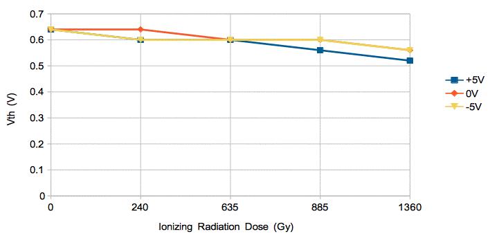
[30-JUN-15] The figure below shows how the threshold voltage of four NDS355AN N-channel mosfets drops with ionizing dose in our Cs-137 chamber. We obtained the plot with four copies of this circuit.

So long as the threshold remains above 0.1V, which is the maximum LO output voltage for our logic chip, our thermometer circuit will work. The minimum un-irradiated threshold voltage of the NDS355AN is 1.0 V, so we can tolerate a drop of 0.9 V, which occurs after 1 kGy. We use the NDS355AN in the thermometer readout of our Bar Head (A2082A). This readout can tolerate 1 kGy without any pre-construction measurements of the threshold voltage. But if we measure the threshold voltage of a random sampling of mosfets, and find them to be 1.6±0.5 V, as we have in the past, our tolerance is at least 2 kGy.
[15-JUL-15] We measure the current gain of ZXTN2031F and ZXTP2025F bipolar transistors at 500-mA collector current after 20 Tn followed by 30 days room-temperature anneal. We bake them at 150°C for 24 hours and measure again. We compare to un-irradiated transistors also. We obtain the results below.

Both transistors have gain greater than 100 after 20 Tn. Their gain recovers significantly during an anneal, which is characteristic of neutron damage.
[30-JUL-15] We build four copies of this circuit to measure the effect of ionizing radiation upon NDS356AP P-channel mosfets. We place the circuits in our Cs-137 chamber, where they receive 6 Gy/hr.

[30-NOV-15] We obtain the following graph of relative transmission through eight optical fibers irradiated by our continuous x-ray source. The four colored plots are for individual fibers. The black plot is the average of four fibers.
All but one of these fibers we received as samples from Brian Rische of Prismian Group, after communicating with CableLan about the darkening of the S705T-02F-62N3 fiber in blue light. As we received them, the fibers were identified as follows. A: "10" 62.5um RH Ge PCVD. B: "11" 50um SRH F PCVD .43 dB/km. C: "5" 50um RH Ge PCVD .44dB/km. D: S705T-02F-62N3. E: Average of four 80-um connectorized fibers.
[05-FEB-16] We irradiate samples of the ZVN3306F mosfet in an SOT-23 package. We mount the package on a SIP adaptor and plug the adaptor into a prototyping board. We apply bias voltages to the gates from −15 V to +15 V. We connect the sources and drains to 0 V. We place the mosfets in front of our continuous x-ray source. Every few days we take them out and measure their threshold voltages. And so we obtain the following plots of threshold voltage versus dose.

The effect of negative bias voltages appears to be similar in magnitude to those of positive bias voltages, so that it is the magnitude of the electric field in the gate oxide that affects the damage, not the direction.

When we put together the final threshold voltages at the end of our irradiation, we obtain the following relationship between threshold voltage and gate bias.

The ZVN3306F is a candidate for use in the radiation-tolerant, low-power analog switches we must include in our Fourteen-Way LWDAQ Multiplexer (A2085)
[07-MAR-16] We subject NDS355AN, UM6K31N, and UM6K34N mosfets to 1.3 kGy in Si with our continuous x-ray source. During the irradiation, each mosfet has its drain and source connected to 0 V and a bias voltage applied to its gate. Every few days we remove the mosfets from the experiment to measure and record their threshold voltages. The figure below shows the drop in threshold voltage for various mosfets and bias voltages. All mosfets took part in an earlier experiment, in which they received roughly 700 Gy. We present these results because they are relevant to our acceptance of our LWDAQ Multiplexer (A2085), which uses the UM6 mosfets for its analog switches.

The NDS355AN is a mosfet we have tested before. The 0.5-V drop in the NDS355AN at 0-V bias is consistent with the change that takes place from 0.7 kGy to 2.0 kGy in our JUN-15 results. The UM6K31N is a 2.5-V mosfet, while the UM6K34N is a 0.9-V mosfet. We see no change in the 0.9-V mosfet's threshold voltage. We plan to repeat this experiment so as to observe the magnitude of the effect in the 0.9-V mosfet.
[01-APR-16] We repeat irradiation of the UM6K34N, measuring its threshold voltage by taking it out of our continuous x-ray room every day or two.
Even with ±5-V gate bias the drop is only 15%, compared to 40% or so for the NDS355AN. During the same experiment, we irradiate a Fourteen-Way Multiplexer (A2085A) to 1.4 kGy, checking it every few hundred Gray to see if it's still working. At 1.4 kGy it captures images on all sockets with no visible degradation of performance. This multiplexer uses the UM6K31N.
[27-APR-16] We receive from UMass Lowell a Fourteen-Way Multiplexer (A2085) and Bar Head (A2082) that received 15 Tn of fast neutrons. We capture images through all multiplexer channels, and from the bar head. We measure power supply voltages on the board. They function normally.
[06-MAY-16] We remove four Black N-BCAM Heads (A2083A) and four Blue N-BCAM Heads (A2083B) from our continuous x-ray source, where they have received 702 Gy at 2 Gy/hr. All boards loop back, take sharp images, and turned on their lasers. Current consumption and laser power remain within the nominal ranges prior to irradiation.
[12-MAY-16] We irradiate a selection of shunt regulators with x-rays. During the experiment, they are biased with a current of a few milliamps. We remove them occasionally and measure their voltage drop.
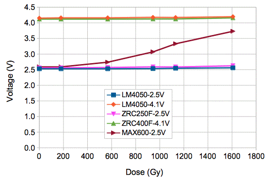
The LM4050 regulators are the ones we use in our newer LWDAQ devices and multiplexers.
[13-MAY-16] We select 4 Black N-BCAM Heads (A2083A) and 4 Blue N-BCAM Heads (A2083B) at random from our recent batches of 440 of each board. We equip them with image sensors and N-BCAM Side Heads (A2074C/D). We arrange them in front of our x-ray source. Because these boards have components on both sides, we must account for absorption of x-rays in the printed circuit board. The image below we took from an ICX424AL after 700 Gy, where the PCB was between the source and the image sensor during irradiation. We see higher dark current in the regions where there was less shielding.

We place a four-layer, 62-mil thick, FR4 printed circuit board, with one ground plane and three signal layers, between our source and a TC255P dosimeter. The dose drops by a factor of four. We arrange two of each type of board with the top side facing the source, and two with the bottom side. We irradiate for one week, accumulating a total dose of 700 Gy in Si for the components on the sides facing the source, and 175 Gy for those facing away. We see no significant change in current consumption when awake or asleep from ±15 V and +5 V. We obtain sharp images from all image sensors. Dark current is consistent with earlier measurements. We see no significant change in laser power.
[16-JUN-16] We measure ionizing radiation tolerance of our original ATLAS camera circuits. The Inplane Sensor Head (A2036) and Proximity Camera Head (A2033A) are vulnerable to ionizing radiation because their DG411DY analog switches are always powered with ±15 V. Their circuits are identical, but their layouts are different. We take four of the A2036 and two of the A2033A and arrange them with half facing towards and away from our x-ray source. We deliver what we believe is 400 Gy in Si to the components facing the source and 100 Gy in Si to those facing away. Later, we find that our x-ray source is operating at 40% of full power, so the actual doses could be as low as 40 Gy and 160 Gy. The boards with the DG411DY facing away are fully functional, but those with the DG411DY facing the source are damaged. The DG411DY can survive at least 40 Gy with ±15 V power applied, but perhaps not 160 Gy. When we replace the three damaged DG411DYs, the boards function perfectly. There is no significant increase in their current consumption. The Inplane Sensor Head (A2047T) and Proximity Camera Head (A2047A) do not use an analog switch. We test two of these, one facing each way, to what we think is 400 Gy, but could be only 160 Gy. They are fully-functional afterwards, with no significant change in current consumption.

[29-JUN-16] We irradiate three N-BCAM BK7 glass lenses with x-rays until they have received 2100 Gy. We see no change in color from start to finish.
[09-SEP-16] We irradiate with x-rays five o-rings we plan to use to secure fiber-optic ferrules in place in the nSW.

In calculating the dose we deliver, we use the absorption spectrum for rubber rather than silicon, and combine the absorption spectrum with our x-ray spectrum. We note, however, that this spectrum we measured for our pulsed source, not our continuous source.
We have been irradiating the A2036 and A2047 in gamma-rays. We summarize our experiments here. The A2047 is the radiation-tolerant version of our ATLAS Proximity Camera Head and In-Plane Head. When powered up but asleep, these circuits fail at roughly 270 Gy, at which point their VHC logic chips are no longer responding to commands. We note that the ATLAS circuits are powered off almost all the time during ATLAS running.
The A2036 fails because one particular part is vulnerable to ionizing radiation: the DG411DY. In one mode of failure, which occurs when the boards are irradiated while they are asleep, the −15 V power switch fails to close when the board wakes up, which occurs because a DG411DY switch fails to open. With only +15 V connected to the op-amps, they draw a total of 250 mA from the +15 V power supply. During the tests, the circuits are either asleep or powered off. When asleep, they have ±15 V connected to the analog switch, but the switches are open. When powered off, the LWDAQ Driver has disconnected its power supplies from its devices, so there is no power connected to the analog switch. When asleep, the A2036 fails after 10 Gy of gamma-rays. We delivered the gamma-rays at two doses: 30 Gy/hr and 3 Gy/hr and obtained the same result. We repeated with circuits we burned in for several days before the irradiation, and obtained the same result. With the boards powered off, they fail after 180 Gy of gamma rays. In the above plot we see the waking current consumption drop as the analog switches fail. This 180 Gy is our best estimate of the radiation tolerance of the A2036 during ATLAS running.

We obtain this plot of the change in threshold voltage of the NDS355AN versus gamma and x-ray dose. The two plots do not agree. The gamma dose appears to be more damaging. We consider the discrepancy between gamma-ray and x-ray damage in this report. But we later discover that our x-ray source is running at 40% of full power. If we reduce the x-ray flux to 40%, the gamma and x-ray effects are in much better agreement: a 1.0-V drop for gammas at 700 Gy and a 0.8-V drop for x-rays at 700 Gy.
[04-NOV-16] We compose the following table summarizing our radiation tolerance measurements so far. We assume the circuits will be operated with their power off almost all the time, as is the case in ATLAS. We use gamma-ray results in preference to x-ray when they are inconsistent.
| Component | Description | Minimum Ionizing Tolerance (Gy) |
ATLAS Ionizing Dose (Gy) |
Minimum Neutron Tolerance (Tn) |
ATLAS Neutron Dose (Tn) |
|---|---|---|---|---|---|
| A2041N | Nine-LED Array for nSW | 1600 | 70 | 16 | 5 |
| A2074C/D | Dual Laser Head for nSW | 1600 | 70 | 14 | 5 |
| A2080A | 36-Way Contact Injector for nSW | 1600 | 50 | 20 | 3 |
| A2082A | Bar Head for nSW | 1600 | 50 | 20 | 3 |
| A2083A/B | N-BCAM Head for nSW | 1600 | 70 | 20 | 5 |
| A2084A | 6-Way Patch Panel for nSW | 1600 | 30 | 20 | 2 |
| A2085A | 14-Way Multiplexer for nSW | 1400 | 50 | 15 | 3 |
| ICX424AL | Image Sensor for nSW | 1400 | 70 | 14 | 5 |
| LXML-PR01 | Royal Blue LED for nSW | 1400 | 70 | 16 | 5 |
| LXZ1-PA01 | Deep Red LED for nSW | 1400 | 50 | 16 | 3 |
| S705T-02F-62N3 | Optical Fiber for nSW | 2500 | 70 | 16 | 5 |
[14-DEC-16] We find that we are running our continuous x-ray source at only 40% of full power. At range 74 cm the dose rate is 1.1 Gy/hr when we expect 2.9 Gy/hr. We increase the voltage to the opto-isolators that drive the x-ray control voltages and obtain 2.9 Gy/hr. We suspect that the opto-isolators have been ageing. The most recent calibration of our x-ray flux was SEP-15.
We irradiate four A2036 circuits in x-rays. They have power connected always, but are asleep except for once per hour when we wake them up and measure the difference between waking and sleeping current consumption. Two circuits have their top side, which is the side with the DG411DY, facing the source. Two circuits have the bottom side facing the source. We measure the dose rate at the location of the circuits with our Radcal ionizing chamber and get 1.1 Gy/hr. The two DG411s facing the source fail at 30 Gy and 33 Gy. The other two boards are still running at 180 Gy.
[19-DEC-16] We irradiate four A2036 circuits in x-rays, arranged as in the experiment above. They have power turned off always, except for a few seconds each hour, when we turn on power and measure the difference between waking and sleeping current consumption. The circuits are at range 74 cm from our continuous x-ray source. We measure dose rate 750 mR/min ≡ 2.9 Gy/hr. After 112 hours, all four circuits are still operational.
[22-DEC-16] We continue irradiating our four A2036 circuits. Two of them have failed, those with the DG411DY analog switch facing the x-ray source.

Failure of the DG411DY takes place after 340 Gy and 337 Gy for No1 and No4 respectively. In gamma rays, we saw failure after a dose of 180 Gy, assuming a dose rate of 3.0 Gy/hr, which is the dose rate in our cesium-137 source that we measured with our ionizing chamber. If we use the manufacturer's calibration of the cesium-137 source at our operating position, the dose rate is 4.3 Gy/hr, in which case the failure occurred at 260 Gy. Within the cesium-137 chamber, we locate our circuits at 18±1 cm, which gives us a ±10% uncertainty in the dose. The calibration of our x-ray source for silicon dose ignores absorption in the plastic package of the DG411DY. The absorption coefficient of carbon for 15-keV x-rays is 0.56 cm2/g, and the density of plastic is around 2 g/cm2, so 1 mm of plastic will absorb no more than 10% of 15-keV x-rays. Our x-rays are at least 15 keV, after passing through our aluminum absorber. We also use a scaling factor to convert ionizing dose in air to ionizing dose in silicon. This factor is 7.6, with uncertainty ±20%. Given all these sources of error in our measurement of absolute dose rate, 340 Gy in our x-ray test is consistent with 180 Gy in our gamma test.
[05-JAN-17] The A2036 No3 in our x-ray irradiation began to fail at around 1.1 kGy. The x-ray source shut down after 1.3 kGy. We re-started, but if turned off again within a few hours at 2.9 Gy/hr. We suspect that the failing No3 is shorting the ±15 V power supplies, and so turning off the x-ray source. Circuit No4 current consumption remains normal. Given that 75% of x-rays are absorbed by the circuit board, it appears that the analog switches on the far side of the circuit board fail at around 300 Gy, which is consistent with the failure of those on the front side at 340 Gy. Later, we run the x-ray source without the damage circuits connected to the LWDAQ and it is stable for a week.
[04-MAY-17] We place a prototype A2080A in our continuous x-ray source, bottom side facing the source at ruler position 100 cm where we measure dose rate 700 mR/min, which implies 2.7 Gy/hr in silicon. We leave power applied to the A2080A. Every hour we turn on each of its four installed Luxeon Z LEDs, deep-red LXZ1-PA01, green LXZ1-PM01, white LXZ2-5770, and royal blue LXZ1-PR01 to power level 7 of 0-10. We also turn on a non-existent LED. In each case we measure the increase in +15V current consumption.
[10-MAY-17] We remove our prototype A2080A after 400 Gy on the bottom side of the board. So far, the buck converter input currents have evolved as shown below.
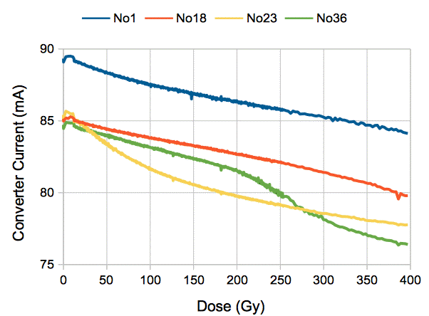
We turn on each LED to power leval 7. We place a 1% neutral density filter over the LED and measure photocurrent with an SD445. For No1, deep-red, we get 1.1 mA, implying 275 mW output power. For No18, green, we get 0.15 mA implying 60 mW. For No23 we get 0.62 mA for white light. For No36 we get 1.13 mA implying 282 mW. Before irradiation, we obtained 310 mW from No36. We have a 9.0% drop in optical power output and a 9.5% drop in current consumption. When asleep, the board consumes 0.5 mA from +15V, 5.0 mA from +5V and 1.3 mA from −15V.
We turn the circuit board around, so that the top side with the LEDs faces the x-ray source at ruler position 80 cm. According to our measurements, the circuit board absorbs 75% of our x-ray dose. The top-side has already received 100 Gy. The source itself is at ruler 16 cm, so our new dose rate will be 4.0 Gy/hr.
[15-MAY-17] Our A2080A has received another 450 Gy of x-rays. The top-side total dose is 100 Gy from the first session and 450 Gy from the second session. The bottom side received 400 Gy in the first session and 510 Gy in the second. The following plot shows buck converter input current rising slightly, reversing the original drop of the first session.

We measure optical output at power level seven as described above. For No1 deep-red 310 mW, No18 green 79 mW, No23 white 0.63 mA photocurrent, No36 280 mW.
[07-SEP-17] We irradiate one Contact Injector A2080A with 14 Tn of fast neutrons in the reactor at UMass Lowell. We now have 35 LEDs and buck converters that have been subjected to the same 14 Tn. The power coupled into a 62-μm core NA=0.22 fiber is 35 μW before irradiation and 22 μW after. But leaving the LED running for 10 minutes the power increases to 28 mW. The next day and several days later, the recovery to 28 μW remains. We believe the self-heating of the LED annealed some of its neutron damage. When we remove an irradiated LED and replace it with a fresh one, we see no significant difference between the performance of an irradiated buck converter and an un-irradiated converter.
[24-JAN-18] We place our 2.4 μCi californium source, Cf-252, up against the window of a TC255P image sensor, cover with black cloth in a dark room, and take an image every two hours with a 100-ms exposure time. The sensor receives a dose rate of roughly 58 1-MeV eq. n/cm2/s, or 35 μTn/week. Pixels damaged by neutron collisions will show up in the images as bright points.
[23-MAR-18] Our TC255P has several bright pixels from neutron damage. We remove the Cf-252, but continue recording images from our TC255P image sensor to see how the dark current generated by the damaged pixels will evolve with time.
[18-MAY-18] We look through thirty thousand ATLAS dark-current images with the help of Inspect_Image.tcl and find roughly one thousand with optical images, or no sensor readout, or corrupted sensor readout. We enhance the BCAM instrument to allow us to select spots with a maximum number of pixels. We find and list bright pixels, dividing them up into files by image sensor name, with Bright_Pixels. We obtain the history of each bright pixel with Pixel_Histories.
[23-MAY-18] We select the sixteen brightest pixels in our neutron-irradiated TC255P. These are the pixels whose brightness is ten or more counts above the average intensity of the image for twenty-four consecutive hours at some time during the 2800-hour image record. With the help of the coordinates of these images, we use Neutron_Hit_Charge to get the net intensity (intensity above average) of these pixels in ever existing image.
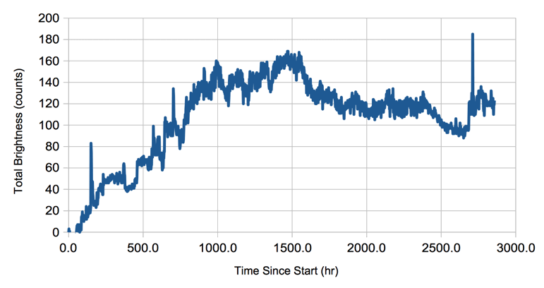
We find the time at which each of these sixteen pixels was damaged, which we call their time of birth. We plot the sum of their intensities versus time since birth. We estimate the dose rate at the image sensor is 60 μTn/wk. The image sensor received roughly 60 μTn/wk for nine weeks, or 540 μTn total.

[30-MAY-18] We turn on our continuous x-ray source. We place our Radcal dosimeter at ruler position range 100 cm from the source (the source is at ruler 16 cm and the dosimeter is at 116 cm). After some rotation of the x-ray tube we measure 460 mR/min = 1.7 Gy/hr at the center of the x-ray cone, which agrees well with our previous calibration, and 430 mR/min = 1.6 Gy/hr at either edge of the cone. At the center of the cone at range 50 cm (ruler 66 cm) we get 1.87 R/min = 7.1 Gy/hr. Our previous calibration at this range was 6.5 Gy/hr. We place a TC255P image sensor at range 50 cm (ruler 66 cm). With the Dosimeter Instrument, threshold "2 $", and 100-ms exposure of the sensor's masked storage area, we obtain charge density 1.0 counts/pixel at the center of the cone and 0.9 counts/pixel on either edge.
[31-MAY-18] We equip a Contact Injector (A2080A) with eight LuxeonZ LEDs of center wavelength 450 nm, 470 nm, 500 nm, 530 nm, 568 nm, 590 nm, 633 nm, and 655 nm. We have seven optical fibers 1.8 m long. Four we made out of our S705T-02F-62N3, named 1, 2, A, and B. Three we received from Fibernet. All have 2.5-mm zirconia ferrules on the ends, named 2821, 2065, and, 2835. We turn each of the LEDs on to full power in turn. We insert one end of each fiber into the injector in the order 1, A, 2821, 2065, 2835, B, 2. We hold the other end 1 mm from a SD445 photodiode and record the photodiode current with a DVM. We place A, 2821, 2065, 2835, and B at range 100 cm from our x-ray source. We turn on the source and leave it over-night. The fibers are receiving 1.7 Gy/hr.
[14-JUN-18] Our irradiation of fibers continues. The dose rate and temperature are well-behaved, and the x-ray AC power remains on, but the LWDAQ turns off the source at random ever few days.

After 230 Gy all five irradiated fibers have transmission 40% compared to start for 450 nm light, and 90% compared to start for 650 nm light.
[03-AUG-18] We have completed our irradiation of optical fibers. The plot below shows the average transmission of the three Fibernet cables and the average transmission of our irradiated S705T cables for deep red light.

We take the average of all five irradiated fiber transmissions and obtain this plot of transmission for all tested wavelengths.

We add the dark current of a larger set of bright pixels in our Cf252 image sensor irradiation. We include any pixel more than five counts above average for a day. Our total intensity us 600 counts at the end of the irradiation period, which is 75 μcount/px/ms. Our isotropic dose calculation and our previous neutron experiments suggest a total neutron damage current of 89 μcount/px/ms.

[23-OCT-19] We find that the attenuition of our eight colors of light in our irradiated fibers is consistent with Rayleigh scattering, as we report in Fiber Irradiation Decay Constant.
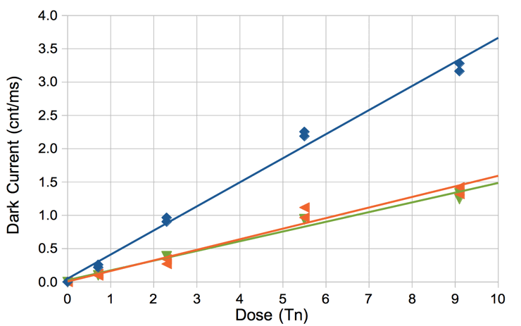
[19-NOV-18] We use dry ice to cool our collection of irradiated ICX424 image sensors to −30°C and measure their dark current, in cnt/ms, with the Dosimeter Instrument as they warm up to room temperature. In order to make sure the portion of the image we are using to measure dark current never contains saturated pixels, we use only the upper half of the image for our dark current measurement. The dark current is proportional to the slope of an image taken in the dark. The Doscimeter Instrument gives us this slope in count/row, which we convert to cnt/ms with 3.0 row/ms.

We capture camera images with two of the irradiated sensors with dark current that drops rapidly to zero at around 0°C. Both sensors provide contrast and definition. The slope of the neutron-damage dark current is roughly one decade per 20°C, or a doubling every 6°C. Our TC255P neutron-damage dark current doubles every 8°C. The TC255P dark current was 0.055 cnt/ms/Tn at 0°C. For the ICX424 we see around 0.2 cnt/ms at 0°C at 15 Tn, or 0.013 cnt/ms/Tn.
[29-NOV-18] Our Cf-252 irradiated image sensor is in the dark at 21°C. We capture images of its storage area with exposure time 0.0 to 1.00 s using this script, which allows 5 s for the sensor to cool down between images.
for {set es 0.00} {$es <= 1.0} {set es [format %.2f [expr $es + 0.02]]} {
  if {![winfo exists $t]} {break}
  set LWDAQ_config_Dosimeter(daq_exposure_seconds) $es
  set result [LWDAQ_acquire Dosimeter]
  LWDAQ_print $t "$es [lindex $result 1] [lindex $result 5]"
  LWDAQ_wait_ms 5000
  LWDAQ_support
}
We obtain the following plot of the intensity of the brightes pixel and the bright pixel charge density. We are using threshold "2 $", which is two counts above the average intensity of the image.
If the bright pixels represent the total dark current in the image from neutron damage, then the neutron-damage dark current is 0.19 counts/px/s, or 190 μcounts/px/ms. From our 1998 irradiation, we expect the following dark current per Tn of neutron dose.
Where D is the dose in Tn and T is temperature in Centigrade. Our sensor has endured 60 μTn/wk for 9 weeks, a total of 540 μTn. Temperature is 21.4°C. We expect the dark current to be 170 μcnt/px/ms. We observe 190 μcount/px/ms.
[11-JAN-19] We take out the eight TC255P image sensors we irradiated with neutrons in the Prospero reactor in 1999.

With each image sensor in the dark we obtain an image from the optical image area (not the storage area). We calculate the vertical slope of intensity in the image, and so obtain a measure of the dark current. Our Dosimeter Instrument gives us slope in count/row. Each row takes 197 μs to read out. The temperature in the lab is 21.6°C. The graph below shows the dark current versus neutron dose for 2019 at 21.6°C and for 1999 at 24.1°C. We have two 20-year old TC255Ps to use for the zero dose.
The new measurement is at a lower temperature. At 24.1°C expect the dark current to be 1.23 times the value 21.6°C. Our damage rate of 0.159 cnt/ms/Tn would be 0.196 cnt/ms/Tn, which is 54% of the damage rate we observed in 1999.
[16-JAN-19] We take out the Prospero image sensors once again and record dark images from the image area. The temperature in the laboratory is 20.8°C. We obtain slope 0.146 cnt/ms/Tn.
[07-FEB-19] We capture the following image with LWDAQ 8.7.2's Dosimeter Instrument from our Cf-252 irradiated image sensor. Pixels more than five counts above the average intensity are marked.

Using a background equal to the average intensity, and a threshold five counts above background, bright-pixel charge density is 1.4 mcnt/px, or 14 μcnt/ms. Temperature is 21.6°C. The dose is 540 μTn. Damage rate is 0.025 cnt/ms/Tn, equivalent to 0.029 cnt/ms/Tn at 20°C.
The following table presents the rate at which neutron dose generates dark current in our various tests. We present two ways to measure the neutron damage. The intensity-slope method uses the vertical gradient of intensity in the image to deduce the average dark current. The bright-pixel method uses the intensity of pixels above background to measure the dark current in the rare bright pixels generated by neutron damage. We use a background equal to the average intensity and a bright-pixel threshold five counts above background.
| Test | Dark Current @ 20°C (cnt/ms/Tn) | Method |
|---|---|---|
| 1998 Lowell, 1 month after | 0.28 | Intensity Slope, 0-8 Tn |
| 1999 Pospero, 1 month after | 0.26 | Intensity Slope, 0-9 Tn |
| 1999 Pospero, 10 months after | 0.23 | Intensity Slope, 0-9 Tn |
| 1999 Pospero, 20 years after | 0.14 | Intensity Slope, 0-9 Tn |
| 2018 Cf-252, 1 year after | 0.029 | Bright Pixels, 540 μTn |
| OCT-2018 ATLAS BCC | 0.078 | Intensity Slope, 0.41 Tn |
| OCT-2018 ATLAS BCC | 0.0035 | Bright Pixels, 0.41 Tn |
We use Dark_Current.tcl to analyze all images in the 20181023 data set, and obtain the following plot of charge density versus slope for the 2596 images.

[09-FEB-19] We note the gap in the above plot for slope values 0.0033 to 0.0047, with the exception of one point at 0.004. We use threshold "5 $ 2 <" on the three data set and see if the gap exists in all three.

[28-MAR-19] We use Slope_Density.tcl to find the average intensity-slope and charge-density of the BCC images in our thirty-five ATLAS dark image sets. We obtain charge density for thresholds 5 to 30 above background, with background equal to the average intensity, and applying gradient-subtraction to the image before finding hits. The charge densities for threshold 5 start to saturate in 2017, where we see more than the maximum 1000 hits in most BCC images. Therefore, we omit the data for threshold 5 in the plot below. Our minimum practical threshold for hit-finding is 10. We convert slope-intensity from cnt/row to cnt/s/px by multiplying by 5080 rows/s, and we convert charge-density from cnt/px to cnt/s/px by multiplying by 10 images/s (each image is a 100-ms exposure). The result is values with fewer leading zeros.

We fit straight lines to the above plots, and ignore the fact that the intercepts are non-zero, to obtain an estimate of the ratio of the slope-intensity to the charge density. We convert slope-intensity to cnt/ms and charge density to cnt/ms so as to obtain a dimensionless ratio.

We have Bright_Pixels.txt, a list of all pixels which at some point have intensity twenty counts above threshold, generated by Bright_Pixels.tcl using thirty-five sets of ATLAS 100-ms dark images. We apply Pixel_Histories.tcl to generate a list of pixel histories. We look through the history with Mention_Histogram.tcl, and obtain the following histogram of the number of times a bright pixel appears in the image sets. Each pixel must appear at least once to be included in the pixel history, and cannot appear more than thirty-five times.

Of 90k bright pixels, 30k appear only once, 10k appear twice, 10k appear 3-4 times, and 40k appear 5+ times.
[21-MAY-19] We present Neutron Damage of CCDs in ATLAS Endcap at CERN.
[23-MAY-19] We find that the latest GEANT4 simulation of neutron dose in the EO layer is in better agreement with our CCD dose measurement, see here.
[27-SEP-19] The pixel histories generated by our Pixel_Histories.tcl have, until now, contained a brightness of zero for any image in which the pixel intensity is below threshold. Our new pixel histories generator fills in these missing brightness values by analyzing the images and measuring the pixel intensity above background. So now our history contains the brightness above background of the pixel regardless of whether it was above threshold or not, and we can see pixels that started at brightness 10 after initial damage, and rose to brightness over 20.
[22-APR-21] We have two Blue N-BCAMs 20MNABNDB00506 and 507 with electronics that have received 300 Gy and 380 Gy respectively, including image sensors, but not including laser driver boards. We mount the BCAMs in the calibration roll cage and take the following image of our fiber source block.

We set daq_subtract_background to 1, so as to subtract background images from our source block images.

We set daq_adjust_flash to 0, so as to stop the BCAM Instrument from increasing the exposure time to get more contrast, which fails because the lower portions of the image start to saturate with dark current. We calibrate both BCAMs twice.

Results of calibration shown below. We have pivot x, y, z (mm), axis x, y, z (mrad), pivot-ccd (mm) and rotation (mrad).
20MNABNDB00506  -10.420 -21.669   0.112  -3.040   0.795   2  50.728 3156.417
20MNABNDB00506  -10.424 -21.669  -0.040  -3.024   0.764   2  50.735 3156.578
20MNABNDB00507  -10.384 -21.677  -1.105   1.823   1.525   2  49.357 3146.985
20MNABNDB00507  -10.375 -21.682  -0.927   1.821   1.532   2  49.354 3146.990
[18-JUN-24] We have an H-BCAM Y71052 in which the front-camera ICX424AL image sensor has two bright pixels that prevent calibration, and in which the rear-camera image sensor has one very bright pixel. We place in our oven at 60°C for sixteen hours. We remove and allow to cool to room temperature. The two bright pixels in the front camera sensor are not visible at 10 ms exposure. The very bright pixel in the rear camera sensor is less bright, but still visible in a 1-ms exposure. We put it back in the oven.
[20-JUN-24] We take Y71052 out of the oven and allow it to cool to room temperature. At 10 ms, looking at a white paper with an ink cross on it, we still see no sign of the two bright pixels in the front camera in 10-ms exposure. The rear camera spot is no longer visible in a 1-ms exposure, still visible in 10-ms exposure.