 Inclinometer Performance
© 2006-2009 Kevan Hashemi, Brandeis University© 2021-2025 Kevan Hashemi, Open Source Instruments Inc.
NOTE: The bi-axial sensor used by this inclinometer is no longer available, other than as it exists in the dozen or so inclinometers we have on the shelf at Open Source Instruments Inc..
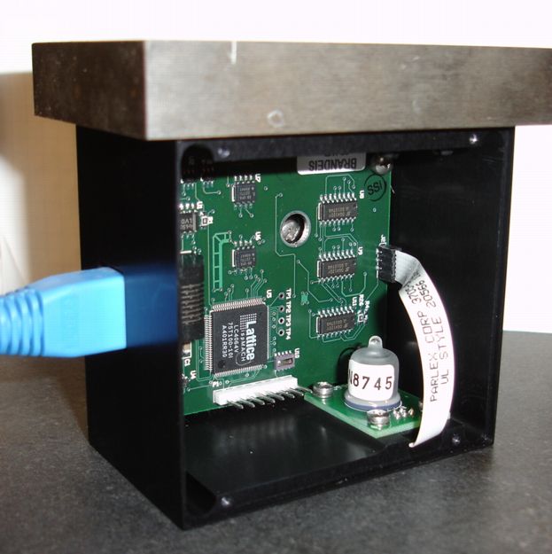
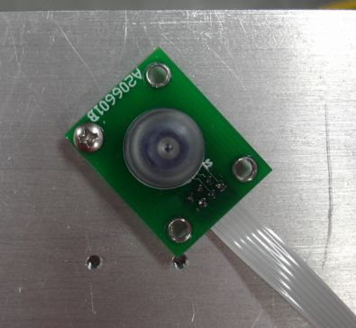
[17-MAY-23] The Inclinometer Head (A2065) allows us to connect a single bi-axial or two uni-axial liquid level sensors to our LWDAQ (Long-Wire Data Acquisition System). The Inclinometer Sensor Head (A2066) connects to the A2065 with a six-way flex cable and provides a 59560D five-pin, glass-body, bi-axial sensor from Applied Geomechanics (no longer in business). The LWDAQ manual contains a section on the Inclinometer Instrument, while the Inclinometer Head manual describes how we drive a bi-axial sensor with a sine wave.
This report starts by presenting our work with the 59560D glass-body, bi-axial sensor. We measure resolution, linearity, stability, and sensitivity to magnetic fields and changes in temperature. The latter half of the report presents our work with the 59577 cermic-body, uni-axial sensor. The ceramic sensor has over ten times the precision of the glass sensor, but accepts the same drive signals. Like the glass sensor, the ceramic sensor is manufactured by Applied Geomechanics.
The liquid-level sensor, drawn here, contains conducting fluid and five pins. There is one center pin and four others arranged symmetrically around it. As we tilt the sensor, the fluid surface remains horizontal, and so ascends up some of the pins, and descends down others. The resistance between two opposite pins is of order a few kilohms. It varies significantly with temperature, and from one sensor to the next. But we are not concerned with the absolute value of this resistance. Rather, we measure the ratio of the resistance between pins. The resistance between two neighboring pins, such as the left pin and the center pin, decreases as the average depth of the fluid between the pins increases. With the sensor horizontal, the resistance between the left and center pins is equal to that between the right and center pins. But as we tilt the sensor to the right, we find that the resistance between the left and center pins is greater than that between the right and center pins. It is this change in the ratio of resistances that gives us a measurement of the inclination of the sensor in both the left-right and front-back directions.
The manufacturer declares that any DC voltage applied across the sensor pins will change the conducting properties of the fluid, and damage the sensor. The Inclinometer Head (A2065) couples all its voltages capacitively to the sensor, to make sure that there can be no DC current circulating in the fluid. We excite the sensor with a sinusoidal waveform instead.
We connect a sine wave to each pair of electrodes in turn, and select the center pin, and both pins, and a ground reference. We digitize the waveforms and determine their amplitude by fourier transform. In our initial consideration of the design, we looked at how the transform of a waveform was affected by noise and innacurate sample frequency. You can do the same, with the help of the LWDAQ tool script you will find here.
The manufacturer claims that these sensors, with their own square-wave based electronics, give stability over several years of 0.2 mrad. We set out to see if we could reproduce their results with our own sin-wave and fourier-transform based electronics and data acquisition system. This Performance Report presents our conclusions so far. You will find a chronological record of our experiments in our Inclinometer Experiments page.
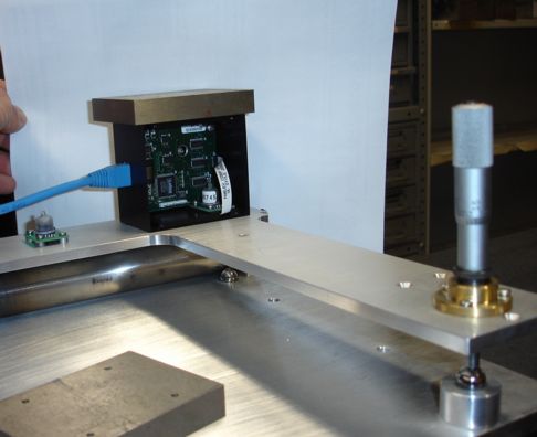
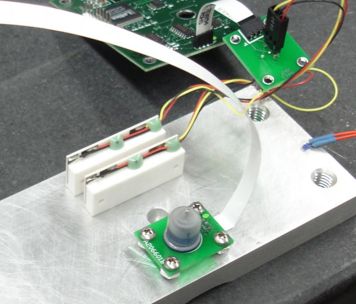
We built a rotation stage for our A2066 tilt sensor, and placed the stage on our granite beam. Also on the rotation stage is a high-precision commerical inclinometer with which we can verify the performance of our own instrument. By rotating the state with its micrometer, we can measure the sensitivity and linearity of our Inclinometer output with inclination.
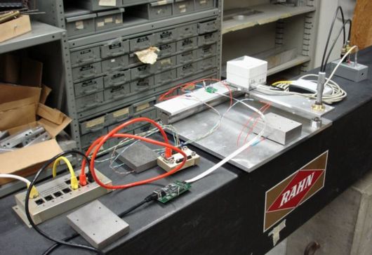
In the figure, you can see a Leica high-precision level, which proved to be accurate and stable to a few tens of microradians. You see cables connecting the Leica to an Input-Output Head (A2057). There are three temperature sensors connected to an RTD Head (A2053). We have the tilt sensor itself, mounted on an Inclinometer Sensor Head (A2066). This is in turn conected via a 6-way 1-mm flex cable to an Inclinometer Head (A2065A).
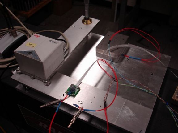
We read out all these instruments together with our Acquisifier Tool. You will find the Acquisifier Script we used here. The micrometer tilts the stage with a lever arm shown here. You will find all our results in an Excel spreadsheet in a zip archive here.
We use X to denote the ratio of the center pin amplitude to the drive amplitude when we drive the X+ pin with a sine wave and ground X−. We use Y to denote the same ratio when we drive Y+ and ground Y−. We use x (lower-case) to denote the rotation of the inclinometer about the axis meaured by X, and y for rotation about the axis measured by Y. We use R to denote the micrometer reading in inches.
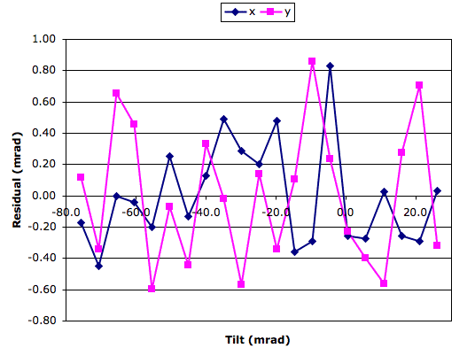
We rotated our sensor in steps of roughly 0.25 mrad and measured Y at each step. The following graph shows residuals from a straight line fit to our graph of y versus inclination. We obtained the true inclination from the Leica instrument. We used the slope of the line to convert residuals in Y, which is a voltage ratio, to residuals in y, which is the inclination.
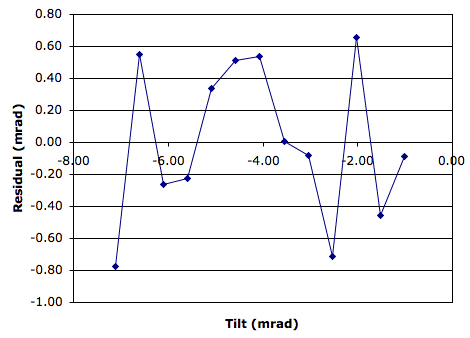
The rms residual in y is 500 μrad. We measured Y with the following parameters set in the Inclinometer Panel: analysis_harmonic = 4, daq_delay_ticks = 12, daq_num_samples = 1709. We performed this experiment with the original eight-bit data acquisition. The resolution of the eight-bit data acquisition was around 400 μrad, compared to 100 μrad for the sixteen-bit data acquisition we adopted later.
A year later, we placed a production-version A2065B Inclinometer on our tilt stage, as shown in the photograph below.
We moved the tilt stage micrometer in steps of 0.05" from 1.00" down to 0.00". For a drawing of the tilt stage, showing the length of the rotation lever arm, see here. These 0.05" steps rotate the stage by 5 mrad in the Y-direction. We did not use the Leica instrument to determine the inclination of the stage. We relied upon the micrometer, which allowed us to cover a greater range. For our results in an Excel spreadsheet, see the A2065B worksheet in Results.zip.
The stage rotates in the inclinometer's y-direction. We define positive rotation in the direction for which the inclinometer's y-measurement increases. The following graph shows the residuals from a straight line fit to our measurements.
The following table gives the properties of the straight line fit, and the resolution in Y and y. One step of 0.05" on the micrometer is close to a 5-mrad change in Y, so the slope in V/V-in is one hundred times greater than the slope in V/V-mrad.
| Measurement | Value | Unit |
|---|---|---|
| Slope | 0.042 | V/V-in |
| Slope | 420 | μV/V-mrad |
| Resolution | 180 | μV/V |
| Resolution | 0.44 | mrad |
We obtained the above graphs using eight-bit data acquisition, whose resolution in x and y is roughly 400 μrad. With the eight-bit data acquisition, the A2065B's linearity is 400 μrad rms over a 100-mrad range (6°)
We recorded measurements from two A2065B Inclinometers and our high-precision Leica inclinometer for over a month. We neglected to record temperature, and we used eight-bit data acquisition instead of the superior sixteen-bit data acquisition. We obtained the following thousand-hour plot of fluctuations in the x and y inclination measured by the A2065Bs.
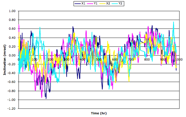
During our experiment, the Leica measurement showed that our granite beam was stable to better than 5 μrad rms. In subsequent long-term tests, we no longer bother to record measurements from the Leica, which we prefer to make available for other experiments. We trust that the granite beam is stable to a few microradians.
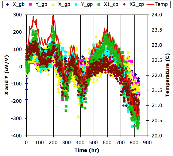
The following graph shows fluctuations in x and y measured with sixteen-bit data acquisition. Also shown is the air temperature and rate of change of temperature above the granite beam.

We see both sensors settling to their final values during the first 100 hrs. One sensor's x measurement rises by almost 3 mrad in the first 100 hrs. From 100 hours to 800 hours, the standard deviation of x and y for both sensors drops below 150 μrad. The temperature in the laboratory changes by ±0.5°C. When the temperature changes by less than 0.1°C/hr, the standard deviation of inclination drops to around 60 μrad.
From 800 hours to 1000 hours, the temperature in the laboratory rises by 3 °C. We see X_1 increase by 600 μrad, while Y_1, X_2, and Y_2 increase by roughly 300 μrad. From 1000 hours to 1100 hours, the temperature drops by 1.5°C and all four measurements drop in proportion. The average temperature coefficient of the tilt measurements is 125 μrad/°C. Our measurements of the effect of Temperature suggest that it is the temperature of the sensor that causes fluctuations in measured inclination, not the temperature of our electronics.
We conclude that the combination of our readout electroncis and the 59560D tilt sensor will provide ±100 μrad resolution so long as ambient temperature remains constant to ±1°C.
For graphs of the effect of cold and heat upon the sensor and our electronics, see the 09-MAY-08 entry in Inclinometer Experiments. Over the course of a thousand hours we observed an apparent sensitivity to temperature in both the X and Y inclinations of an 59560D sensor of 125 μrad/°C (see Stability.)
Applied Geometrics drives their liquid-level sensors with a square wave applied to two adjacent pins and zero volts applied to the two remaining pins. We, on the other hand, apply a sine wave to one pin only and zero volts to the pin opposit. We leave the adjacent pins open-circuit. We show the geometry of both driving methods in the drawing below. In the four-pin drive, the direction of current through the sensor fluid is at 45° the current we see with the two-pin drive. The X and Y rotation directions for these two drives are at 45° to one another.
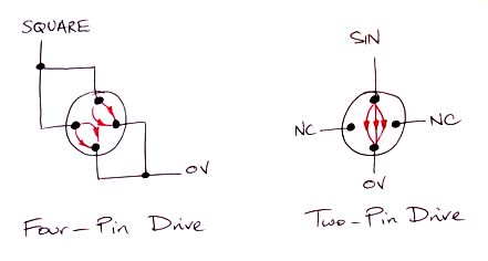
Applied Geomechanics prefers the four-pin drive. We prefer the two-pin drive. The advantage of the two-pin drive is that the current density through the resistive fluid is greater at the center of the sensor, where the center pin is located. Because the current density is greater, the sensor sensitivity to changes in the current is greater. We varied R (as shown here) from 0.40" to 1.10" in 0.05" steps. These steps correspond to a rotation of roughly 5 mrad. We measured the ratio of center pin amplitude to drive amplitude at each step for four different driving voltage arrangements.
| Description | SIN | VCOM | A2065_commands | Orientation | Slope (μV/V-mrad) |
|---|---|---|---|---|---|
| Two-Pin on X | X+ | X− | 0094 0093 0095 | 0° | 7 |
| Two-Pin on Y | Y+ | Y− | 008E 008B 008F | 0° | 410 |
| Four-Pin on X and Y | X+ Y+ | X− Y− | 0086 0083 0087 | 45° | 300 |
| Two-Pin on X | X+ | X− | 0094 0093 0095 | 45° | 280 |
We began with our two-pin drive on X and the sensor oriented as shown here. We drive X+ with SIN, connect X− to VCOM and leave the Y-pins disconnected. The slope in X is small because we are rotating in the y-direction. We apply two-pin drive to the Y-pins. We drive Y+ with SIN, connect Y− to VCOM, and leave the X-pins disconnected. We obtain a slope of 410 μV/V-mrad. Now we turn the sensor, as shown below, so that our stage will rotate it in the optimal direction for the four-pin drive.
We rotate the sensor in steps and measure the slope in X and Y. We expect the slope to be the previous slope in Y divided by sin(45°), or 290 μV/V-mrad. We measure a slope of 300 μV/V-mrad. Now switch to four-pin drive and measure the slope in X. We drive X+ and Y+ with SIN, and connect X− and Y− to VCOM. The slope we obtain in Y is 280 μV/V-mrad. We turn the center about a vertical axis and confirm that this 45° orientation is indeed the one in which we obtain the maximum slope in Y for the four-pin drive.
We conclude that the maximum slope for the two-pin drive is 410 μV/V-mrad, while the maximum slope for four-pin drive is only 280 μV/V-mrad. We will continue using the two-pin drive.
We placed an A2065B on our granite beam, as shown below, weighted down with a steel slug, as shown above. We picked it up, shook it, and re-placed it on the beam ten times. Each time we measured the inclinometer's x and y outputs within one second of replacing the inclinometer on the beam. We used eight-bit data acquisition, so we expect an inherent 500-μrad stochastic error due to the eight-bit digitizaion. We obtained the following results.

We repeated our experiment, but waited thirty seconds after each re-placement before we measured x and y.
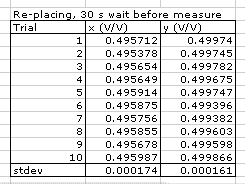
In both experiments, the standard deviation of X was 170 μV/V and of Y was 300 μV/V. Using the slopes we obtaine in our linearity section, these ratios correspond to inclination resolutions of 400 μrad and 700 μrad.
We conclude that the short-term re-mounting resolution of the A2065B is better than 1 mrad. Over the long-term, we know that sensors can drift by up to 3 mrad in a hundred-hour period, as shown here.
Here we consider the effect of stochastic, electronic noise, otherwise known as white noise upon the phase measurement made by the Inclinometer Instrument. The instrument takes N uniformly-spaced samples of the inclinometer waveform, f, and determines the amplitude of the harmonic with period T samples.
where n is the sample number, A(T) is the amplitude of the harmonic with period T, and f(n) is the value of the inclinometer waveform at sample n. This formula will give A(T) = 1 for f(n) = sin(2πn/T) provided that N/T is an integer.
Suppose we add a random disturbance e(n) to each of our samples, and that this disturbance has zero mean and standard deviation η. The change in A will be given by the same formula, but with e(n) used in place of f(n). The mean change will be zero. The standard deviation of the change will be 2η/N times the sum in quadrature of sin(2πn/T) for all 0 ≤ n ≤ N-1. If we assume that N/T is an integer, the standard deviation comes out to be η√(2/N).
In practice, our inclinometer waveform will be subject to both white noise and quantization noise. Quantization noise results from converting a continuous voltage into a digital number. A quantum is the voltage range covered by each digital value. Quantization noise is evenly-distributed across one quanta, and has standard deviation q/√12, where q is the quantum size. Even though quantization noise is not guaussian, the effect of many quantization disturbances is guassian, in accordance with the central limit theorem.
We verified our stochastic noise formula by adding quantization noise of various amlitudes to pure sinusoidal waveforms, and measuring the standard deviation of the fourier term as we changed the noise. We obtained the following results.
| N | T | η | σ | σ/(η&radic(2/N) |
|---|---|---|---|---|
| 400 | 10 | 0.03 | 0.001838 | 0.9 |
| 400 | 100 | 0.00003 | 0.000002 | 1.0 |
| 400 | 100 | 0.0003 | 0.000020 | 1.0 |
| 400 | 100 | 0.003 | 0.000232 | 1.1 |
| 400 | 100 | 0.03 | 0.001637 | 0.8 |
| 400 | 100 | 0.3 | 0.019068 | 0.9 |
| 400 | 400 | 0.3 | 0.023726 | 1.2 |
| 400 | 400 | 0.03 | 0.002726 | 1.3 |
| 400 | 400 | 0.003 | 0.000239 | 1.2 |
| 4000 | 4000 | 0.03 | 0.000738 | 1.1 |
| 40 | 40 | 0.03 | 0.005918 | 0.9 |
The table shows that our formula works well. Note that the number of complete periods in our sample set does not change the effect of stochastic noise.
The inclinometer center-electrode waveform has a typical amplitude of 0.2 V. Our eight-bit ADC's input range is 1 V, so its quantization noise is 1 mV rms. If we have N = 6836, we expect amplitude measurement noise of 17 μV. We also have the same noise on the input-electrode waveform, which has typical amplitude 0.4 V. When we divide the two measured amplitudes, quantization results in an error of roughly 100 μV/V rms. If we use N = 1709, we can expect a 150 μV/V rms error.
Our samples are not synchronous with the inclinometer waveforms. We set the sample frequency and the number of samples so that we get a whole number of harmonic periods in our sample interval. But our samples do not take place at the same exact phase of the harmonic in consecutive measurements. Quantization noise could be random from one sample to the next. We are not sure. If it is random, we see that its magnitude is large enough to make it the dominant source of stochastic error in the inclinometer measurement. If it is not random, we see that it will vary with the offset voltages in the analog signal path. These offset voltages vary with temperature, so we would see variation in apparant inclination with changes in temperature. But this variation would not scale with temperature. It would be cyclic or random when plotted against temperature.
With a 16-bit ADC, we would get a factor of 256 reduction in quantization noise.
Historical Note: The LWDAQ Driver (A2037) provides an 8-bit ADC and a 16-bit ADC. Starting with Firmware Version 13, the LWDAQ Driver with Ethernet Interface (A2037E) allows exactly-timed sampling with the 16-bit ADC. Earlier versions of the firmware allowed exact timing only with the 8-bit ADC. During our first two years of work with the Inclinometer Head (A2065), we used the 8-bit ADC. But the calculations we performed above motivated us to create Firmware Version 12 and try out the 16-bit converter.
The LWDAQ Driver (A2037)'s adc16 job digitizes the LWDAQ analog return voltage with 16-bit precision. The adc16 job completes when the delay timer has counted to zero and the ADC conversion is complete. The ADC conversion takes somewhere between 8 μs and 10 μs, depending upon the particular A2037E and its operating temperature. Starting with A2037E firmware version 13, the delay timer starts counting down at the start of conversion. Provided that the count-down takes longer than the conversion, the count-down will dictate the sample period. This period will be 375 ns plus 125 ns per delay count. We set the delay count in the Inclinometer Panel using the delay_ticks parameter. If we set delay_ticks to 100, the sampling period will be exactly 12.875 μs.
The inclinometer waveform is 32.768 kHz divided by 28, which is 1.1703 kHz. The waveform period is 854.49 μs. The accuracy of our Fourier Term amplitude measurement depends upon our having a whole number of waveform periods in our sample interval. The following piece of Pascal code searches through the possible combinations of daq_delay_ticks and daq_num_samples for ones that provide a sample interval very close to a whole number of 854.49-μs periods.
program p;

const
  period=854.49;
  half_period=period/2;
  base=0.375;
  tick=0.125;
  threshold=0.07;
  max_periods=20;

var
  num_samples,num_periods,delay_ticks:integer;
  best,error,sample_time:real;

begin
  for delay_ticks:=100 to 800 do begin
    for num_samples:=100 to 1000 do begin
      sample_time:=(base+delay_ticks*tick)*num_samples;
      error:=period*(sample_time/period-trunc(sample_time/period));
      if error>half_period then error:=period-error;
      num_periods:=round(sample_time/period);
      if (num_periods<=max_periods) and (error<=threshold) then
        writeln(delay_ticks:10,num_samples:10,num_periods:10,error:10:2);
    end;
  end;
end.
The program produces the following list of combinations.
| daq_delay_ticks | daq_num_samples | analysis_harmonic | Remainder (μs) |
|---|---|---|---|
| 106 | 439 | 7 | 0.05 |
| 116 | 517 | 9 | 0.04 |
| 122 | 875 | 16 | 0.04 |
| 132 | 557 | 11 | 0.02 |
| 172 | 625 | 16 | 0.04 |
| 184 | 329 | 9 | 0.04 |
| 194 | 347 | 10 | 0.03 |
| 194 | 694 | 20 | 0.05 |
| 216 | 437 | 14 | 0.02 |
| 326 | 187 | 9 | 0.04 |
| 344 | 197 | 10 | 0.03 |
| 344 | 394 | 20 | 0.05 |
| 391 | 347 | 20 | 0.05 |
| 434 | 219 | 14 | 0.02 |
| 436 | 109 | 7 | 0.05 |
| 514 | 119 | 9 | 0.04 |
| 554 | 135 | 11 | 0.02 |
| 622 | 175 | 16 | 0.04 |
| 691 | 197 | 20 | 0.05 |
After some experimentation, we settle upon new default Inclinometer Instrument settings of daq_delay_ticks = 132, daq_num_samples = 557, and analysis_harmonic = 11. With these values, we obtain X and Y resolution of 20 μV/V, or 50 μrad, which is five times better than we obtained with our 8-bit ADC, even though we are using ten times fewer samples.
One potential application for our A2065B Inclinometer is at CERN in the ATLAS pit, measuring the shape of the floor. We estimate the field strength near the floor to be less than 0.1 Tesla (1000 Gauss). The field will be stable with time, but may vary by up to 0.1 T/m. We performed our own magnetic field tests to determine whether the A2065B and purpose we built an electromagnet with a gap designed to accommodate the 59560D tilt sensor are suitable for use in ATLAS.
We built an electromagnet and set up a Hall-Effect magnetic field sensor. We calibrated the electromagnet and the sensor, as we describe the Hall Probe section of our experimental record. The field in the center of the air gap of our electromagnet was 50 mT. We placed a tilt sensor in the field and turned on the magnet current. In Electromagnet we show how the effect of the heat generated by the electromagnet masked any effect of the magnetic field.
We switched to a cold magnet made of permanent neobynium magnets and a C-clamp, as we describe in Cold Magnet. The air gap in our cold magnet had field 50 mT at the center, rising to 300 mT at the edges. With the cold magnet, we were able to affect the inclination measured by our tilt sensor by ±1.4 mrad, as we show in Magnetic Effect.
The pins of our tilt sensor are magnetic. We measured the attractive force between a neobynium magnet pressed up against the sensor glass, and calculated how much the sensor pins must bend in response to this force. We found that the pin-bending in fields of between 100 mT and 1 T is large enough to cause 1-mrad changes in measured inclination. We arrived at the following Rule of Thumb.
Rule of Thumb: Magnetic fields up to 100 mT affect the measured inclination by less than a hundred microradians. Fields between 100 mT and 1 T can cause milliradian changes in measured inclination, depending upon the orientation and gradient of the field. Fields stronger than 1 T are almost certain to affect the measured inclination by several milliradians.
We are not the first to measure the effect of magnetic fields upon Applied Geomechanics liquid-level inclinometers. Dr. Todd Johnson of Fermilab studied the effect of magnetic fields upon Applied Geomechanics liquid level sensors. We received a report on his results from Gary Holzhausen, and we keep a copy of the report here. Dr. Johnson used static magnetic fields and concluded that a s10 T/m gradient produces a 500-μrad change in measured inclination. Our observation was that a 30 T/m gradient produces at 1.4-mrad change. It appears at first that we agree with Dr. Johnson. But Dr. Johnson was working with a larger, 755-1150, high-gain tilt sensor. The 755-1150 sensor has resolution 1 μrad, while our smaller 59560D has resolution 100 μrad. If our theory of pin-bending is correct, field gradients should have a smaller effect on larger sensors because the pin bending is less significant compared to the separation of the pins.
A group at the CIEMAT research institute in Spain followed Dr. Johnson's study. We keep a copy of their report here. The CIEMAT group found that the sensitivity of the sensors to magnetic field gradient increased with the strength of the magnetic field. Their plots are, however, ambiguous to our eyes: the units of magnetic field gradient are "Gauss" instead of "Gauss/mm", and we're not sure which of their various lines correspond to which field strength. They do not state clearly which sensor they used to perform their tests. Nevertheless, we are not surprised by their claim that the effect of gradient increased with field strength. As the field strength increases to 1 T, the permeability of the sensor pins increases by a factor of ten, thus increasing the effect of the same gradient by a factor of ten. We can also understand their observation that it takes a while for the sensor to settle in a new field: we found it hard to avoid distorting the environment of the pin when we applied a strong magnetic field. We had to weigh down our sensor with aluminum blocks on a granite table to avoid such movements.
We conclude that the A2065A with 59560D tilt sensor will perform well in the 100-mT residual fields outside the ATLAS detector, but that fields of 1 T or higher are likely to cause 1-mrad errors in measured inclination.
We took ten Inclinometer Sensor Heads (A2066) and measured their sensitivity to rotation in x and y using our rotation stage. We used our two-pin drive and sixteen-bit ADC with daq_delay_ticks = 132, daq_num_samples = 557, and analysis_harmonic = 11. The average slope of X with rotation was 412.9 μV/V/mrad. The average slope of Y was 413.4 μV/V/mrad. The standard deviation of slope was 12 μV/V/mrad. The standard deviation of the difference between the x and y slopes was 4 μV/V/mrad. The standard deviation of repeated measurements of the slope of the same sensor was also 4 μV/V/mrad.
From this we conclude that the x and y direction slopes of any given sensor agree to better than 1%. From one sensor to the next, the slope varies by 3% rms, with a spread across our ten samples of 10%.
We measured the height of the fluid in the sensors. Our experimenter, Miles Ketchum, reports, "It's a little difficult to get the measurement of the depth due to the nature of the glass they used, but measurements of the 13 remaining unsoldered sensor heads range from 2.26 mm to 1.95 mm, with a standard deviation of .10 mm which is about 5%."
A 5% variation in fluid depth will give a 5% variation in sensitivity. We suspect that the variation in x and y slope from one sensor to the next is dominated by variation in the fluid depth. If we want to use the A2065A to measure changes in inclination with accuracy ±5%, we can do so without measuring the sensitivity of individual sensors. But if we want ±1% accuracy, we must measure the sensitivity of each sensor.
[25-MAR-09] We begin work with the 59577 ceramic sensor. We soon find that we can drive two of them using one A2065B circuit board. We glue two ceramic sensors and a glass sensor to a plate with a thermometer and measure stability on our granite beam.
We connect two ceramic sensors to one A2065B using an adaptor with two three-pin connectors soldered on either side of one of our A2066B circuit boards. We place a 250-μm shim under the plate, 140-mm from the thermometer end. We insert and remove the shim and measure X for the two ceramic sensors and Y for the glass sensor. The sensitivity of the glass sensor Y is 407 μV/V-mrad, which is close to the value of 420 μV/V-mrad we obtained with more careful measurements. The sensitivity of the ceramic sensors is 6800 μV/V-mrad and 6400 μV/V-mrad.
We take a hundred measurements over a few minutes. The resolution in X of the ceramic sensors is 30 μV/V, and in Y for the glass sensor is also 30 μV/V. Using our approximate slopes, these values translate to angular resolutions of 4 μrad for the ceramic sensors and 70 μrad for the glass sensor.
After 800 hours, we see a near-perfect correlation between X1_cp and temperature, and a strong correlation between X2_cp and temperature. We see the same correlation with the four voltage ratios we obtain from the two glass sensors as well, from both the X and Y ratios. The correlation is −170 μV/V/°C. With a total of 4°C variation in temperature, all sensors provide stability of roughly 100 μV/V rms. From this we claim that the A2065B combined with the ceramic sensor has resolution 15 μrad rms for ±2°C. The A2065B combined with the glass sensor has resolution 240 μrad for ±2°C.
We report in more deteil in Ceramic Sensor.
[17-MAY-23] With sixteen-bit data acquisition, the resolution of our A2065B Inclinometer with the 59560D bi-axial sensor is roughly 60 μrad over the short-term and 120 μrad over the long-term. Changes in ambient temperature degrade the instrument's resolution. To obtain long-term resolution of 100 μrad, we must ensure that the sensor temperature remains stable to ±1°C. The sensor is far more sensitive to temperature gradients across its width than it is to absolute temperature. To attain 100-μrad resolution, the ambient temperature should change no faster than 0.1°C/hr. Nevertheless, by taking the average of twenty-four hourly measurements, the A2065B Inclinometer provides a daily measurement accurate to 100 μrad even with a ±5°C daily temperature cycle. The linearity of the A2065B with 59560D is better than 0.5% over a 100-mrad range (we observed 400 μrad rms residuals). We find the sensitivity of the sensors to inclination to be consistent to within 10%. Individual calibration will be necessary if we are to measure changes in inclination with 1% accuracy. Magnetic fields of less than 100 mT have no observable effect upon the tilt sensor. But stronger fields can affect the measured inclination by several milliradians. The Inclinometer (A2065B) with 59560D can provide 500-μrad accuracy in a laboratory with no attention paid to laboratory temperature. In a temperature-stabilised clean room, the same instrument will provide long-term accuracy of 100 μrad. In an experiment hall with ±2 °C variations, and magnetic fields up to 100 mT in the sensor fluid, the A2065B will provide long-term accuracy of 300 μrad or better.
Having said that, our Implantable Inertial Sensor (IIS) contains the BMA423 micropower acceleromater, which claims to have capable of providing acceleration resolution of 1 mrad. Higher-power, more expensive solid-state accelerometers can probably deliver inclinometer performance equal to or better than the instrument described above, at a lower cost. We will be happy to design such an instrument for the LWDAQ.