Inclinometer Experiments

Note: For an introduction to our liquid-level inclinometer, and a description of our apparatus and early work on the instrument, see Inclinometer Performance. Here we record our day-to-day work on the instrument from February 2008 onwards. We provide some section headings just to make it easier for us to navigate the page. But the results remain in strict chronological order.

Contents

Dummy Sensor

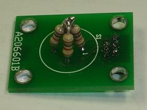
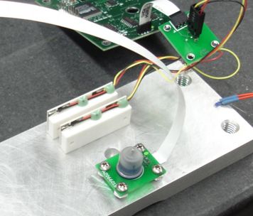
[21-FEB-08] We resolve to measure the fundamental resolution of the A2065 circuit by substituting a dummy sensor for the liquid level sensor. We make the dummy sensor with resistors, as shown below.

Figure: Dummy Sensor. We create our X signal with two 1-kΩ resistors, and our Y signal with two 10-kΩ resistors.

We find that the resolution we obtained from the dummy sensor was no better than that we obtained with the liquid sensor. We tried a few changes to the circuit. We increased R7 and R8 by a factor of ten to improve decoupling on VCOM (see schematic). This had no effect. We increased the number of samples and periods of the sinusoid we recorded with the Inclinometer Instrument. The increases had a strong effect. We took ten samples under each of a variety of conditions and determined the resolution of the instrument X and Y in each case. Our data is in the Dummy Sensor sheet of Results.xls, here.

We see that our resolution with both the dummy and liquid sensors improves by more than a factor of two when we increase the number of periods by a factor of four. A resolution of 60 μV/V corresponds to 0.15 mrad (0.008°). But note that the resolution with our dummy sensor is no better than that with the liquid sensor. We change the default Inclinometer Instrument settings to analysis_harmonic = 16, daq_delay_ticks = 12, daq_num_samples = 6836.

[21-FEB-08] We start acquiring from two A2065Bs. One has the dummy sensor attached, the other a liquid sensor. Both are on our granite beam. We add a thermometer as well, and record measurements ever hour. For the A2065Bs we use the superior 6836-sample, 16-period data acquisition settings. Our Acquisifier script is here. Our results are in the spreadsheet called Dummy Sensor, here.

Figure: Stability of Dummy Sensor and Liquid Sensor with Temperature, Using 8-Bit ADC. The Xdm and Ydm graphs give X and Y recorded from the dummy sensor. The Xlq and Ylq graphs give X and Y recorded from the liquid-level sensor.

[25-FEB-08] We see clear correlations with temperature. The dummy sensor measurements are less stable than the liquid level measurements. We suspect a problem with the dummy sensor's Inclinometer Head (A2065).

[12-MAR-08] We make a new dummy sensor out of 0.1% wire-wound 1-kΩ resistors for X and 5% 10-kΩ resistors for Y. We switch over to the 16-bit ADC, using a LWDAQ Driver (A2037E) with firmware version 13, in which we can obtain precise sample intervals with the driver's sixteen-bit converter. We use analysis_harmonic = 11, daq_delay_ticks = 132, daq_num_samples = 557. We heat and cool the senor with a heat gun and freezer spray, and see changes of up to 1 mrad/°C, but we cannot obtain consistent graphs of apparant inclination with temperature. We resolve to let the dummy and liquid sensors run over-night, to see the effect of the slow 0.5°C over-night drop.

Figure: Stability of Dummy Sensor and Liquid Sensor with Temperature, Using 16-Bit ADC. The Xdm and Ydm graphs give X and Y recorded from the dummy sensor. The Xlq and Ylq graphs give X and Y recorded from the liquid-level sensor.

Cross-Talk

[13-MAR-08] The standard deviation of the liquid sensor measurement over-night, and with a 0.5-°C drop, is 60 μrad in both directions. The dummy sensor performs poorly. Its measurements drift together, and we suspect they are correlated with temperature in the same way they were in our longer-term test with the 8-bit ADC. We resolve to try a new Inclinometer Head (A2065).

We take out a new circuit and perform the following experiments.

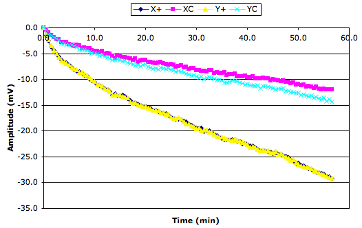
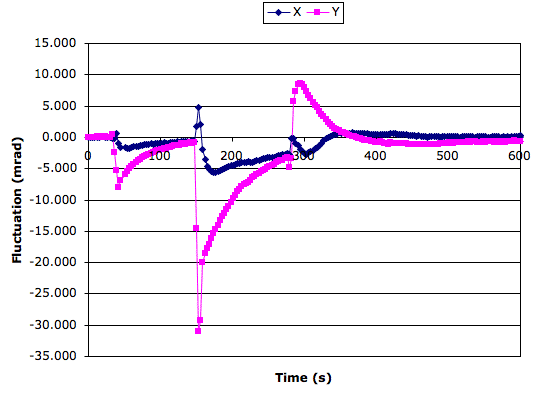
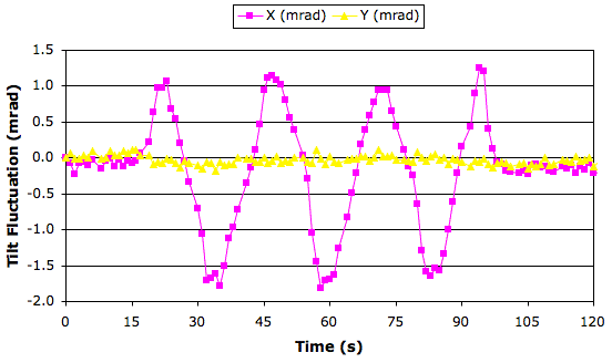
Our center-electrode signal is being corrupted by cross-talk. With no sensor and no flex cable, the center-electrode signal has amplitude 41 mV. This amplitude increases when we add a cable, and increases further when we touch the cable. This cross-talk affects X and Y equally. If the cross-talk amplitude changes, X and Y will together, just as they did in the graph above. We set up our new circuit with no sensor and no cable, and watch it for an hour. We obtain the following extraordinary plot.

Figure: Cyclic Fluctuations with No Sensor, Using 16-Bit ADC. Graphs Xdm and Ydm for no sensor, Xlq and Ylq for liquid sensor. We acquire Xdm and Ydm first.

We reverse the order of the data acquisition, so that we read the liquid sensor first and then the test circuit: no effect. We obtain the same graph from the test circuit. The shared cyclic fluctuation in X and Y has period 10 minutes and peak-to-peak amplitude 1.1 mrad. We make a more detailed recording, as shown below.

Figure: Amplitude Fluctuations Recorded from Test Circuit with No Sensor. Graphs X+ and Y+ are the input amplitudes for the X and Y directions, and XC and YC are the center electrode amplitudes.

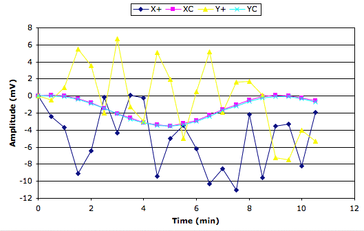
The cyclic variation in center-electrode amplitude is obvious. Its period is 10 minutes and its peak-to-peak amplitude is 4 mV. When we divide 4 mV by the X+ amplitude of 8 V, we obtain a 500 μV/V change in X, which corresponds to a 1.2 mrad change in apparant inclination.

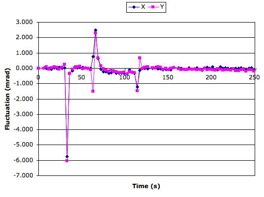
We start changing things to see if they affect the amplitude of this sinusoid. We increase A2065_settling_delay from 0.05 s to 0.5 s: no effect. We notice that we are using a 15-ft CAT-5 patch cable for the test circuit, but a 15-ft LWDAQ branch cable for the liquid sensor circuit. So we switched the patch cable for a branch cable: no effect. Go back to previous test circuit, on in a box with lid off, with no sensor plugged in: period of the cyclic variation in XC and YC increases to 30 minutes, but amplitude remains 4 mV.

We switch back to the test circuit with the 10-minute period and switch to daq_num_samples = 219, daq_delay_ticks = 434, and analysis_harmonic = 14: no effect. Try daq_num_samples = 439, daq_delay_ticks = 106, and analysis_harmonic = 7: no effect. We modify the firmware so that the sinusoidal frequency runs independently from the circuit's ring oscillator. Up until now, we synchronised the 32.768-kHz reference clock to the local ring oscillator and used the synchronised clock to generate the sinusoids. We re-programmed the test circuit: no effect.

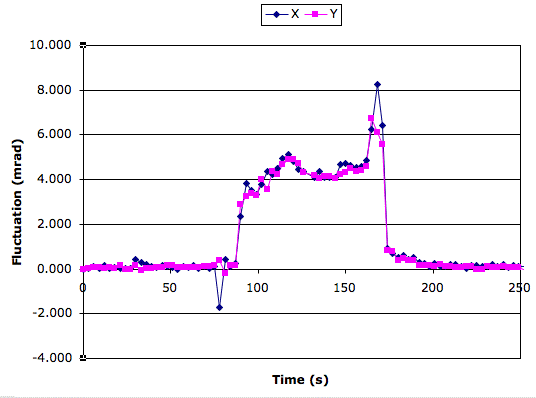
It's time to go home, so we leave the Acquisifier running over-night, taking data from the test circuit, liquid sensor, and thermometer.

Figure: Stability of Dummy Sensor and Liquid Sensor with Temperature. Xdm and Ydm are from test circuit. Xlq and Ylq are from the liquid-level sensor. We shook the liquid sensor before we began taking data. The test circuit has no sensor or cable plugged in.

[14-MAR-08] We obtain the graph above. The standard deviation of the liquid sensor reading drops to around 50 μrad after the first few hours. The cyclic error in the test circuit remains strong and steady.

Decouple VCOM with a 10-μF capacitor (see schematic): no effect. Decouple ±15V power supplies: no effect. Replace R26 with a solder lump: XC amplitude drops from 41 mV to 0 mV and cycle drops from 4 mV to 0 mV. Replace R26 with 10 kΩ: XC amplitude drops from 41 mV to 0.5 mV and cycle drops from 4 mV to <0.1 mV. On the oscilloscope, we see other asynchronous clock frequencies superimposed upon the fundamental 1.17 kHz. We believe that it is the interaction of these clock frequencies with the fundamental and the clock on the driver that give rise to the cyclic changes in cross-talk amplitude. But we are not certain.

With no sensor attached, the voltage on CTR is cross-talk induced upon the PCB traces, and loaded by R26. When we decrease R26 from 1 MΩ to 10 kΩ, we load the cross-talk voltage source and attenuate it by a factor of almost 100. The source impedance of the cross-talk is around 1 MΩ. When we plug a sensor into the board, the sensor's impedance loads the cross-talk. The sensors's AC impedance is much lower than its DC impedance. With a voltmeter we measure 2 MΩ between adjacent pins. But with a sensor plugged in and R26 = 1 MΩ, the XC amplitude is 2.296 V. With R26 = 10 kΩ, the XC amplitude is 2.161 V. The impedance between CTR and VCOM presented by the sensor at 1 kHz is around 600 Ω.

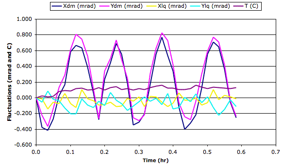
We now understand why the A2065 performs better with a sensor plugged in than with no sensor. We put two fully-assembled Inclinometers on our granite table and check for cyclic errors. We obtain the graphs below from the newly-connected Inclinometer. We see the amplitude of the waveforms decreasing by about 0.5% over the first hour.

Figure: Start-Up Changes in Waveform Amplitudes. This is for an Inclinometer with tilt sensor, connected to the LWDAQ just before we began recording. We see no sign of cyclic changes in the waveform amplitudes.

Resolution

[16-MAR-08] We leave the Inclinometers running.

Figure: X and Y Inclination over Weekend for Two Sensors. Sensor 1 had been sitting sideways in a box until we placed it on the beam and connected it to our data acquisition system. Sensor 2 had been sitting on the beam, connnected to the data acquisition system for weeks. But we disconnected it and carried it around briefly before the experiment.

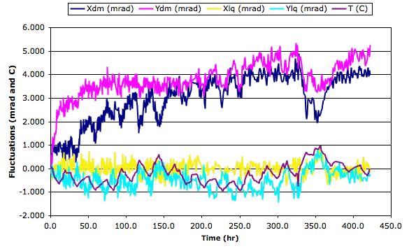
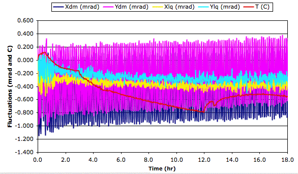
[18-MAR-08] We suppose that Sensor 1 is settling, while Sensor 2 was settled prior to the start of our experiment. The measurements of Sensor 2 are stable to 70 μrad rms. We will leave the instruments running for another week. Looking at the X_2 graph, we see that the effect of temperature is of order +100 μrad/°C. The effect upon the remaining graphs is too small to observe.

[11-APR-08] We add the derivative of temperature with time to the plot, and see how the jumps in inclination are associated with jumps in temperature, not the absolute value of the temperature.

Hall Probe

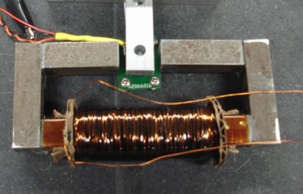
[24-APR-08] We made ourselves an electromagnet with an air gap just large enough for a tilt sensor, as shown in the picture below.

Figure: Home-Made Electromagnet. Shown are (1) the epoxy-encapsulated coil, (2) the iron core, (3) the air gap with tilt sensor, and (4) the hall probe.

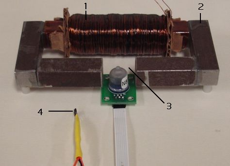
The hall probe is an A1301 from Allegro. We connect the hall probe to an Input-Output Head (A2057), which supplied 5-V for the sensor and reads the sensor output. With a 5-V supply, the sensor output is nominally 2.5 V at zero field, and varies by 2.5 mV/Gauss. The Earth's magnetic field is roughly 0.5 Gauss (50 μTesla). We fixed the hall probe to a rotation stage, oriented it straight up, and rotated it in 30° steps to confirm its sensitivity to the Earth's magnetic field.

Figure: Hall Probe Output versus Orientation. The maximum occurs when the front side of the probe is facing north. the minimum occurs when it faces south.

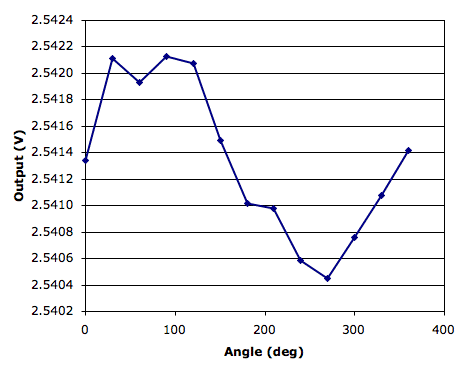
We know the approximate direction of north in our laboartory, and it corresponds to the maximum sensor output. The total change in output as we rotate the sensor is 2 mV. If the sensor sensitivity is 2.5 mV/G, this gives the strength of the Earth's magnetic field as 0.4 G, which is about right. We will translate hall probe voltage into magnetic field by subtracting 2.5413 and dividing the result by 25 V/T (T is for Tesla, 1 Tesla = 10,000 Gauss).

We attach a power supply to the electromagnet. We put the positive voltage on the lead that emerges at an inner corner of the core. We place the hall probe at the center of the air gap with the front face to the left. We increase the coil current form zero, and obtain the following plot.

Figure: Field Strength versus Current. We measure the field strength at the center of the air gap in our electromagnet.

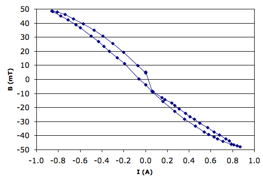
We see hysterisis caused by residual magnetism in the iron. The field strength in the gap reaches a maximum of 50 μT. Our objective is to determine the effect of fields of order 10 μT upon the tilt sensor. Fields of 10 μT are the approximate strength we see a few meters outside 1-T magnets like those of the ATLAS detector.

Heat Cycles

[30-APR-08] We stop the long-term stability test in preparation for some forced cooling and magnetic fields. We note that the temperature coefficient of the measured inclinations is positive for all four coordinates, and roughly 200 μrad/°C.

[09-MAY-08] We separate the tilt sensor from the Inclinometer Head (A2065A) with a 20-cm flex cable. We place the sensor on our granite beam in its metal enclosure and hold the enclosure down with a 1-kg weight. We record the inclinometer fluctuations with time as we cool the sensor with dusting gas, freeze it with freezer spray, and heat it with a heat gun.

Figure: Inclination Fluctuations with Changes in Sensor Temperature. The sensor starts off at a uniform 20°C. At time 30 s, we spray the sensor with dusting gas, which cools it to approximately 10°C. At 150 s, we use a short burst of freezer spray to cool the sensor to approximatly −30°C, and coat it with frost. At 280 s, we blow hot air upon the sensor and heat it to approximately 50°C.

We see the exponential settling of the measurement after a sudden change in temperature. The absolute value of the sensor temperature has a direct and significant effect upon our measurement.

With the sensor once again at thermal equillibrium, we apply the same three temperature shocks to the Inclinometer Head (A2065A), taking care not to affect the sensor.

Figure: Inclination Fluctuations with Changes in A2065 Temperature. We subject the A2065 to dusting gas, freezer spray, and hot air.

The thermal shocks have a large effect upon our measurements while they are taking place, but no significant effect within seconds of the shock ending. We conclude that the absolute value of the temperature of the A2065A has no significant effect upon our measurement. In the y-direction, we observe an effect of order 0.3 mrad/°C. In the x direction the effect is much smaller, and changes sign above room temperature.

We remove the lid of the LWDAQ Driver (A2037E) and subject its sixteen-bit analog input amplifier, filter, and digitizer to the same three thermal shocks.

Figure: Inclination Fluctuations with Changes in A2037E Temperature. We subject the A2037E to dusting gas, freezer spray, and hot air.

The frost left by the freezer spray affects the A2037E circuits until we evaporate the frost with hot air, at which point our measurements return to their original values. We conclude that the absolute value of the temperature of the A2037E has no significant effect upon our measurement.

Electromagnet

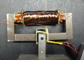
[09-MAY-08] We set up our electromagnet and an isolated tilt sensor as shown below.

Figure: Sensor in the Electromagnet on Granite Beam

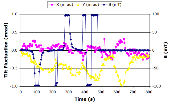
We recorded the following graph, which shows the effect of changing the current through the electromagnet and moving the electromagnet. We used a Acquisifier script Inclinometer_3.txt.

Figure: Steps in Magnetic Flux Density. We vary the magnetic field by changing the coil current and by moving the coil away from the sensor.

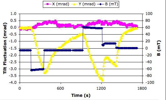
The first step in B we cause by running 900 mA through the electromagnet in one direction. The coil starts to get hot. The y inclination, which is abour the axis parallel to the magnetic field, is strongly affected with what appears to be the beginning of an first-order response. The x inclination is weakly affected. We turn off the current. The y inclination starts to return towards its starting value. We reverse the magnetic field by running 900 mA through the electromagnet in the opposite direction. y starts off in the same direction it did before. The direction of the magnetic field does not affect the direction of the effect upon y. We wonder if the change in y is caused by heating instead of the magnetic field. We move the magnet away from the sensor while leaving the current on. The y inclination begins to move rapidly back towards its starting value. After twenty seconds, we move the magnet a few millimeters closer to the sensor, so as to increase the field strength while causing no significant increase to the heat received by the sensor from the coil and the yoke. This slight movement of the coil causes y to start dropping again. We move the coil another 30 mm away and y turns around and heads towards its starting value, approaching the starting value asymptotically.

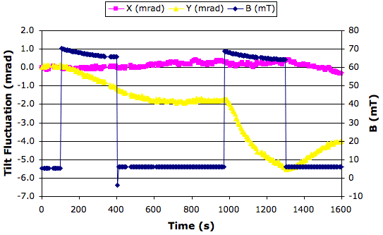
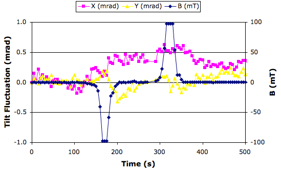
We place a thermal shield made out of paper between the electromagnet and the tilt sensor, as shown below.

Figure: Heat Shield Around Sensor.

We measure inclination and field every five seconds. We turn on the electromagnet. We see y drop 1.3 mrad in 300 seconds, or 4 μrad/s. We turn off the magnet. We see y stops dropping. After a few minutes, we remove the thermal shield and turn on the electromagnet. Now y drops 3 mrad in 200 seconds, or 15 μrad/s. We turn off the magnet. We plot our measurements in the graph below.

Figure: Steps in Magnetic Flux Density. The first application of magnetic field is with a heat shield around the sensor. The second application is without a heat shield.

We conclude that the large drop in y when we turn on the electromagnet is the result of the front face of the sensor being warmed by the electromagnet. The front face is on the Y− side of the sensor (see layout). The x measurement is less affected than y because the x pins are equidistant from the magnet coil.

Cold Magnet

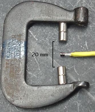
[12-MAY-08] We make a cold magnet out of a c-clamp and some small, permanent magnets, as shown below. The magnets are part number 469-1003 at Digi-Key, and are manufactured by Radial Magnets. They are 0.25" in diameter and 0.25" long, and we believe they are made of Neodenium. The field strength at the flat surfaces of the magnets is out of the ±100 mT range of our Hall Probe. At the center of the gap in our cold magnet, the field strength is 50 mT. Away from the center, the field rises to 100 mT, after which our Hall Probe saturates. According to Radial Magnets, the field at the surface of these neodenium magnets is around 400 mT.

Figure: Cold Magnet. We use four small

We place our Hall probe on one side of the tilt sensor and move the gap of the cold magnet forwards until it encloses the sensor. We are holding the magnet by hand. We withdraw the magnet, reverse it, and move it up. All this time we are holding the magnet with one hand. We set aside the magnet and hold our hand around the sensor, starting at time 580 s. We move our hand away at around 630 s.

Figure: Cold Magnet Held with Warm Hand. Shown are field intensity on the X− face of the sensor, saturating at 100 mT, and x and y from the sensor with time.

The graph shows that our warm hand has a larger effect upon the sensor than the magnet. We repeat our experiment, with the cold magnet held at the correct height with a piece of metal. We touch the magnet only to move it towards and away from the sensor..

Figure: Cold Magnet Near Tilt Sensor. Shown are field intensity on one side of sensor, saturating at 100 mT, and x and y from the sensor with time.

We see a smaller effect in y, but a larger effect in x. The Hall Probe is pressed against the X− side of the sensor (see layout). If the Hall Probe heats the sensor, we would expect a decrease in x. We see an increase in x two minutes into our experiment.

[13-MAY-08] We move the Hall Probe away from the sensor. We let the sensor settle for half an hour. We start recording. After 60 s, we lower the magnet into place around the sensor. At time 120 s we remove the magnet. At time 180 s, we replace it in the opposite orientation. At time 240 s, we remove it, and at 300 s we end our recording.

Figure: Cold Magnet and Tilt Sensor. At time 0 s there magnet is far from the sensor. At time 60 s we place the north pole next to the sensor's X+ pin and the south pole next to X−. The field at the X+ and X− pins is roughly 100 mT. At the CNTR pin the field is 50 mT. At time 120 s we remove the magnet. At time 180 s we restore the magnet, but with opposite field direction. At time 240 s we remove the magnet. The standard deviation of x and y is 60 μrad.

It took us a while to obtain the above results. We encountered several minor practical difficulties in presenting the magnetic field. For example, if we slid the magnet into position horizontally, the magnetic field would pull on the steel screws we used with the aluminum standoffs of our Inclinometer Sensor Head (A2066). This pull would give us sudden changes in x of order 500 μrad. In the end, we lowered the magnet into place, with the center of the gap aligned with the center pin of the sensor.

Magnetic Effect

We placed the cold magnet around the sensor, resting upon an aluminum plate that we could slide from side to side at a distance. We started with the gap field centered upon the sensor, with the north pole next to X−. We started taking measurements. We moved the cold magnet towards X+ until the south pole almost touched the glass of the sensor. We moved it back to the other extreme. We repeated this process several times. We left the magnet centered upon the sensor. The following graph shows the effect of the changing magnetic field upon the sensor.

Figure: Cold Magnet and Tilt Sensor. The field at the X- pin varies from roughly 300 mT down to 50 mT while the field at X+ varies from 50 mT to 300 mT.

We put more weight upon the sensor to make sure it was not tilting, and repeated the experiment. We obtained the same result.

We now consider whether our magnetic forces can bend the steel pins sufficiently to cause the apparant changes in x shown in the graph above. The pins in our sensors are magnetic. We can pick up a loose sensor with one of our neodymium magnets. With the help of a weighing scale, we measure the force exerted by two of our neodynium magnets upon a sensor pin when the magnet is pressed up against the glass in front of the pin. The force is roughly 10 g weight, or 100 mN.

The steel pins of the 59560D are 10 mm long, but only 5 mm protrudes into the glass cell, and our magnet is only 6 mm in diameter. The 100 mN is distrubuted along the 5 mm length of the pin. Let us assume that this distributed 100 mN causes the same bending as 50 mN on the tip of the pin. The pins are 0.5 mm in diameter (we measured them and checked the data sheet). They are made of steel. The Young's Modulus of steel is 200 GPa.

We looked at the bending of circular wires elsewhere, and arrived at the conclusion that the radius of curvature of a circular cantilever is:

r = Ed⁴/60T,

where r is the radius of curvature, E is Young's Modulus, d is diameter, and T is the torque. In this case, T ≈ 50 mN × 5 mm = 0.25 mN-m. The radius of curvature of the pin is roughly 800 mm. The tip of the steel pin is displaced by 800 mm × (1 - cos(5 mm/800 mm)) = 16 μm. Only the first 2 mm of the pin is in the sensor fluid. Where the pin breaks the surface, it is displaced by only 2.6 μm. The average displacement of the pin in the fluid is 0.9 μm. The outer pins of the 59560D lie on a 6.35-mm diameter. The distance through the sensor fluid from X+ to CNTR is roughly 3000 μm. When our magnet pulls upon X+, this distance changes by an average of 0.9 μm, or 290 ppm, which will cause our X voltage ratio to change by 290 μV/V. The response of X to inclination is 410 μV/V-mrad, so a 290 μV/V change in X represents a 580-μrad change in x.

In practice, we observe a total change in x of 2.7 mrad as we bend X+ and X− alternately. Half this change is 1.4 mrad. Our estimate of the change in x caused by close proximity of one of our neodynium magnets is no better than an order of magnitude estimate. The effect is proportional to the fourth power of the pin diameter and the square of the fluid depth. If the fluid depth is 2.5 mm instead of 2.0 mm and the pin diameter is 0.45 mm instead of 0.5 mm, the change in x will be 1,400 μrad instead of 580 μrad.

The displacement force experienced by a steel pin in a magnetic field is proportional to the gradient of the magnetic flux density. With our cold magnet close to the sensor, the maximum gradient we can obtain is roughly 300 mT over 10 mm, or 30 T/m. But the steel pin also experiences a torque in a magnetic field, and this torque is proportional to the magnetic flux density itself, not the gradient. It is this torque that moves a compass needle. We determine the torque by differentiating the magnetic field energy in the pin with respect to the angle it makes with the field lines. We assume that the pin generates its own magnetic flux density, parallel to its axis, of Bsinθ, where θ is the angle the axis makes with the external field. This assumption is good enough for our order-of-magnitude estimate. The energy of the field generated by the pin is:

E = B²sin²θ V/2μ,

where V is the volume of the pin. When we differentiate this energy with respect to angle, we get torque:

T = B²sin(2θ) V / 2μ

In a 300-mT field, μ is of order 0.003 (see here), so the torque in our 0.5-mm diameter 10-mm pins when they are at 45° to a 300-mT field will be roughly 0.1 mN-m. This torque is less than the 0.25 mN-m we estimated will result from the force on the top of our pin combined with its being anchored in the center. Nevertheless, it is clear that both the torque generated by the flux density and the force generated by the flux density gradient are of the right order of magnitude to cause our apparant changes in x.

So far, we have ignored the fact that the permeability of iron varies dramatically with field strength, as shown here. In particular, the permeability increases sharply from 0.002 H/m to 0.01 H/m as the field strength 40 A/m to 60 A/m (see Magnetic Field for difference between magnetic field strength and magnetic flux density). The torque on a pin might be 100 times larger in a 500-mT field than in a 50-mT field. Indeed, we observe that a 50-mT field has less than a 100-μrad effect upon the sensor, but a 300-mT field has a 1-mrad effect.

We propose the following rule of thumb for the five-pin 59560D.

Rule of Thumb: Magnetic fields up to 100 mT affect the measured inclination by less than a hundred microradians. Fields between 100 mT and 1 T can cause milliradian changes in measured inclination, depending upon the orientation and gradient of the field. Fields stronger than 1 T are almost certain to affect the measured inclination by several milliradians.

Ceramic Sensor

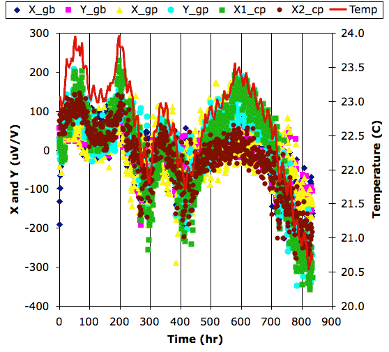
[02-APR-09] We analyze 140 hours worth of samples from the setup shown here and described in Ceramic Sensor. We obtain seven plots, as shown here. Graphs X_gb and Y_gb are X and Y from a the glass bi-axial sensor in the black box resting on the beam. Graphs X_gp and Y_gp are form the glass bi-axial sensor on the plate. Graphs X1_cp and X2_cp are X for the two ceramic sensors on the plate. The final graph is ambient temperature. The sensitivity of the ceramic measurements, X1_cp and X2_cp, is 6800 μV/V/mrad, and of the glass measurements is 420 μV/V/mrad.

The temperature ranges over 1°C and shows twenty-four hour cycles. We see that the glass sensors are stable to around 60 μV/V, or 140 μrad, which is what we expect with such variations in temperature. The ceramic sensors appear to drift by 700 μV/V, or 100 μrad. The drift correlates with temperature. The standard deviation of the difference between the two ceramic sensors is 70 μV/V, or 10 μrad.

[28-APR-09] We repeated the above experiment after the sensors had spend a month settling down on the granite beam, and obtained this plot. In one twenty-four hour period, the two ceramic sensor appear to detect the same 180-μrad change in inclination. We rotated the connector of X1_cp so that real rotations of this sensor should appear with opposite polarity to those of X2_cp. We confirmed that tilting the plate causes changes of opposite sign in X1_cp and X2_cp. Electrical errors will remain of the same polarity. We leave the system running, taking one sample per hour.

[01-MAY-09] We obtain this graph, in which we see a shared drift for X1_cp and X2_cp, which suggests that it is not the sensors that are generating the drift, but rather our electronics. We switch the circuits used by the glass sensor and the ceramic sensor.

[05-MAY-09] With the switched electronics, the X1_cp and X2_cp measurements are stable to 41 μV/V and 37 μV/V respectively, while the X_gp and Y_gp measurements are stable only to 118 μV/V and 85 μV/V respectively. You will find the latest plots here. Our initial poor resolution with our ceramic sensors can now be blamed upon the particular A2065 we used to drive them. The standard deviation of X1_cp and X2_cp is 40 μV/V, which suggests a resolution of 6 μrad.

Figure: Stability of Various Sensors in Test Stand. The sensitivity of the ceramic measurements, X1_cp and X2_cp, is 6800 μV/V/mrad, and of the glass measurements is 420 μV/V/mrad.

[11-MAY-09] We take a look at the X_gp circuit. It is circuit number WP16. The only thing that distinguishes it from other A2065Bs is a quantity of flux residue around the R4 and R26 footprints (see schematic). The R4 footpring is empty. We cleanded off the flux and restored the circuits to their previous positions. We will monitor X_gp for a week to see if the WP16 circuit is still noisy.

[23-JUN-09] The X_gp measurement is still noisy. There is something wrong with that particular A2065B but we do not yet know what is wrong. Meanwhile, we obtain 70 μV/V resolution with the ceramic sensor over two weeks. We changed the A2065B attachd to the glass sensor on the plate, and started a new run.

[24-JUL-09] After another 600 hours we obtain 70 μV/V resolution with the ceramic sensor, or 10 μrad. We see good correlation between temperature and the changes in one sensor, but not the other. The sensors are mounted in opposite directions on the aluminum plate. In one sensor, distortions of the plate with temperature will be of the same sign as electronic temperature effects, and in the other sensor the two effects will be of opposite sine.

Figure: Stability of Various Sensors in Test Stand. The sensitivity of the ceramic measurements, X1_cp and X2_cp, is 6800 μV/V/mrad, and of the glass measurements is 420 μV/V/mrad.

[01-SEP-09] After 800 hours, we see a near-perfect correlation between X1_cp and temperature, and a strong correlation between X2_cp and temperature. We see the same correlation with the four voltage ratios we obtain from the two glass sensors as well, from both the X and Y ratios. The correlation is −130 μV/V/°C. With a total of 4°C variation in temperature, all sensors provide stability of roughly 100 μV/V rms. From this we claim that the A2065B combined with the ceramic sensor has resolution 15 μrad rms for ±2°C. The A2065B combined with the glass sensor has resolution 240 μrad for ±2°C.

If we compensate for temperature by −130 μV/V/°C, our resolution improves to 45 μV/V (7 μrad) for the ceramic sensors and 60 μV/V (140 μrad) for the glass sensors. In our Electronic Errors section below, we try to find the source of the temperature correlation.

Electronic Errors

[28-JUL-09] Although the ceramic sensor continues to perform well, our new A2065B on the glass sensor of the plate performs poorly, as you can see here. We resolve to discover the source of these problems. Using the apparatus shown here, we changed the long flex connector we were using with the noisy electronic board for a short flex connector. We still obtained poor performance in X_gp and Y_gp, as shown here.

We have three A2065Bs in our setup, numbers 13WP, 17WP, and 22WP. It is 13WP that is noisy. The previous noisy circuit we threw away. Circuit 13WP has R5 = 330 Ω, while 17WP and 22WP have 470 Ω. We changed R5 on 13WP to 470 Ω and tried again.

[31-JUL-09] The increase in R5 eliminates the problem with board 13WP. The increase in resistance decreases the amplitude of the returned signal, which means the sinusoid does not get cut off at the top. Before the increase in R5 the returned sinusoid appeared to be nearly clipped, but not quite. Our two days of data are here.

[01-SEP-09] We appear to have a −130 μV/V/°C relationship between any voltage ratiio we measure with our A2065B and the temperature of its sensors. The same relationship applies to both glass and ceramic sensors.