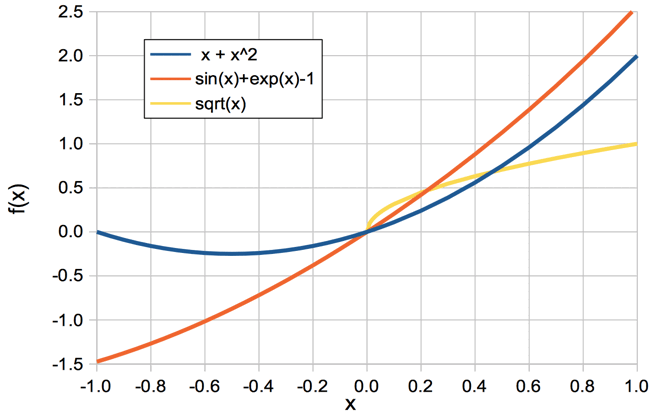
Figure: Example Functions of x. We do not plot f (x) = √y for x < 0 because the square root of a negative number is an imaginary number, and our graph allows us to plot only real numbers.
[11-DEC-23] This text serves as a introduction to infinitesimal calculus for science and engineering students. We take time to introduce the fundamental concepts of infinitesimal calculus, and illustrate these with numerical calculations and geometry. We proceed through differential equations and integrals with brief mathematical discussions followed by detailed examples of their application. Our intention is to teach calculus by showing calculus at work. We trust that the interested student will fill in their own table of derivatives and integrals as they proceed in their scientific endeavors. What we want to do is demonstrate how calculus allows us to advance our understanding of the physical world. In our text, we have attempted to be as brief as possible. In order to comprehend the text, solve every single exercise in each section before you move on to the next.
Let x be a real number. We say x ∈ ℝ. Consider the expression x + x2. How does its value vary as x gets smaller?
| x | x + x2 | Difference |
|---|---|---|
| 1 | 2 | 100% |
| 0.1 | 0.11 | 10% |
| 0.01 | 0.0101 | 1% |
| 0.001 | 0.001001 | 0.1% |
| 0.0001 | 0.00010001 | 0.01% |
As x gets smaller, the expression x + x2 gets closer to x. The x2 part becomes insignificant. At some point, x + x2 becomes indistinguishable from x. We may not agree about when we can first ignore the x2 part, but as we keep making x smaller, we will eventually be forced to agree that there is no significance difference between x and x + x2. The fact that x2 becomes insignificant compared to x for very small values of x is a fundamental principle of infinitesimal calculus. We say x is infinitesimal when we allow its value to approach zero, but never actually reach zero, and we write x→0. To express the behavior of x + x2 as x→0 we say, "The limit of x + x2 as x→0 is x."
A function of x is a mathematical expression whose value depends on x. The expression x + x2 is a function of x. We use the notation f (x) to indicate a function of x. The function need not provide a value for every x, but it must provide only one value for a given x. The function √x is the positive square root of x, so that √9 = 3, not −3. The same √x does not return a real value when x = −1. Nor does the function 1/x return a numerical value when x = 0. When the value of a function is always a real number, we say it is real-valued, or f (x) ∈ ℝ.
When we determine the limit of f (x) as x→0, we are seeking to produce an answer that contains one and only one term in x. If we consider the function 1 + x2, its limit as x→0 is also 1 + x2. It is true that the function becomes arbitrarily close to 1 as x→0, but the point is not the determine the value of the function as x→0, but rather to summarise how the value of the function changes as x→0. In this case, the change in the function as x→0 is represented entirely by the term x2. But if we have the function 1 + x + x2, its limit as x→0 is 1 + x. The variation represented by x2 is negligible compared to the variation represented by x.
Example: What is the limit of sin(x) as x→0? Here, we assume that x is in radians, so that sin(π/2) = 1. We set our calculator to work with angles in radians, and get sin(0.01) = 0.0099998, which is only 0.002% different from 0.01, so the limit of sin(x) as x→0 is x.
Example: What is the limit of ex as x→0? We enter exp(0.01) on our calculator and get 1.01005, which is close to 1.01, so the limit of ex as x→0 is 1 + x.
Exercise: What is the limit of (x + x4) as x→0?
Exercise: What is the limit of (1 + x) as x→0?
Exercise: What is the limit of (1 + 1/x) as x→0?
Exercise: What is the limit of cos(x) as x→0?
Let f (x) be a real-valued function of x ∈ ℝ. We could have f (x) = x + x2, or f (x) = sinx + ex − 1, or f (x) = √x. We plot each of these functions below.

Consider f (x) = x + x2 in the plot above. For each value of x, the function f (x) has a value. At x = 0, we have f (x) = 0. When x = 1, we have f (x) = 2. The slope of the line varies also. If we imagine a ball on the line at x = −1, the ball would roll to the right. We say the slope of f (x) at x = −1 is negative, or downwards. At x = 1, the same ball would roll to the left. We say the slope of f (x) at x = 1 is positive, or upwards. So long as the graph of f (x) versus x is smooth (that is: has no infinitely sharp corners), we can approximate small sections of the graph with short, straight lines. The smaller the sections, the better the approximation. In the figure below, we see a close-up of f (x) = x + x2. We let y = f (x) for brevity. In the close-up, x increases from x to x + δx, and y increases from y to y + δy. Here we use δ to mean "a small change in".
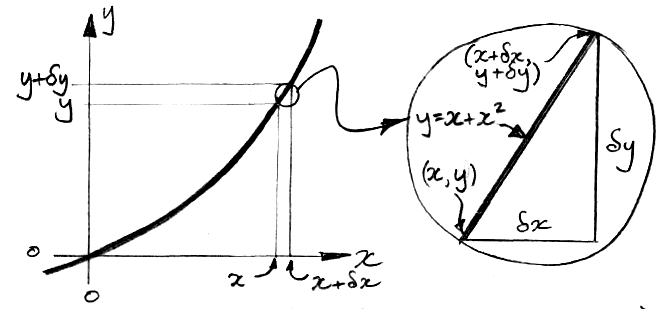
When we increase x by δx, y increases by δy. The slope of the line in the close-up is defined as δy/δx. We have y = x + x2, so we can find δy in terms of x, and so determine the slope as a function of x and δx.

Now let δx→0 and we obtain the slope in terms of x alone, because as δx→0, the term in δx becomes vanishingly small compared to 1 + x.

As δx→0, the slope depends only on x, not δx. It turns out that this is true for any smooth function of x. The limit of the slope as δx→0 is the derivative of y with respect to x, written dy/dx. It is the slope of the graph of y in an infinitesimal neighborhood of x.
Example: When x = −0.5, our equation predicts that the slope will be zero, and indeed the slope is zero in our plot of x + x2 above. We also predict that the slope will be +1 at x = 0 and +2 at x = 1. An examination of the same plot shows that these predictions are also correct.
We can also write df (x)/dx for the derivative of f (x) with respect to x, and we can write d(x + x2)/dx to mean the derivative of x + x2 with respect to x.
Example: What is the derivative of x2 with respect to x? Let x increase to x + δx. We have x2 increasing to (x + δx)2 = x2 + 2xδx + (δx)2. Subtract x2 to get δ(x2), which is 2xδx + (δx)2. Divide by δx to get slope δ(x2)/δx = 2x + δx. The limit of the slope as δx→0 is d(x2)/dx = 2x.
Exercise: What is the derivative of y = x3 with respect to x?
Exercise: What is the derivative of y = 6x with respect to x?
Exercise: What is the derivative of y = 5 with respect to x?
Exercise: What is the derivative of y = x3 + 6x + 5 with respect to x?
Exercise: What is the derivative of y = ex with respect to x? Use eδx = 1 + δx as δx→0 and recall that ea + b = ea eb.
To differentiate a function with respect to x is to calculate its derivative with respect to x. When we differentiate f (x) = x + x2 with respect to x, we obtain df (x)/dx = 2x. The derivative is another function of x. We denote this derivative function f '(x), where the single mark indicates "differentiated once with respect to x". Because f '(x) is itself a function of x, we can differentiate it and obtain f ''(x) = d(2x)/dx = 2. The function f '(x) is the first derivative of f (x) and the function f ''(x) is the second derivative. We can also write f ''(x) as d2f (x)/dx2. The third derivative of f (x) is d3f (x)/dx3 = f '''(x). In our example, f '''(x) = 0. The higher derivatives after that are all zero also.
Rule: When f (x) = xn for any real number n, we have f '(x) = nxn−1.
Example: Let f (x) = x5. Then f '(x) = 5x4, f ''(x) = 20x3, f '''(x) = 60x2, f ''''(x) = 120x, f '''''(x) = 120, and f ''''''(x) = 0.
Consider the function f (x) = x3 and its derivatives, shown below. As x increases from −3, the slope of x3 decreases until it reaches zero at x = 0. After that, the slope increases again. We say the graph of x3 undergoes an inflection at x = 0.
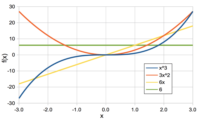
The slope of x3 is given exactly by the plot of 3x2. Looking at 3x2, this graph also has a slope, and its slope is always increasing. For x < 0 the slope is negative, at x = 0 the slope is 0, for x > 0 the slope is positive. We say the graph of 3x2 is at a minimum at x = 0. The slope of 3x2 is given exactly by the plot of 6x. Looking at 6x, we see it has its own constant slope, and this slope is given by the last line in the plot: the constant value 6.
Exercise: What is the derivative of f (x) = 2x3 + 4x2?
Exercise: What is the derivative of f (x) = e4x? Use eδx = 1 + δx as δx→0 and recall that ea + b = ea eb
The derivative of a function is zero when the function reaches a maximum, an inflection, or a minimum. The second derivative is negative at a maximum, zero at an inflection, and positive at a minimum.
Exercise: At what value of x does the function f (x) = x2 − 2x have a minimum?
Exercise: Find any minima, maxima, or inflections of the function f (x) = x3 − 2x2.
The rules of differentiation are mathematical relationships that help us obtain the derivatives of complicated functions. We can derive the rules ourselves with the addition of δx to x, but the proofs take long enough that the rules are worth remembering.
Power Rule: When f (x) = g(x)n for any real number n and any other function g(x), we have f '(x) = ng'(x)g(x)n−1.
Example: Let f (x) = (3-x2)2. Then f '(x) = −4x(3−x2).
Example: Let f (x) = √x. Well, √x = x½ so f '(x) = ½x½−1 = ½x−½ = 1/(2√x).
Exercise: If f (x) = 1/x, what is f '(x)?
Product Rule: When f (x) = g(x)h(x), we have f '(x) = g'(x)h(x) + g(x)h'(x).
The product rule is easy to prove, so we will so so here. We can use the product rule to prove the power rule, but the proof is a little more sophisticated.
Derivation of the Product Rule: Suppose f (x) = g(x)h(x), the product of two other functions of x. For a small increase δx in x we have f (x + δx) = g(x + δx)h(x + δx). But g(x + δx) is just g(x) + δx.g'(x): the change in g(x) is the slope of g(x) multiplied by δx. So we have f (x + δx) = [g(x) + δx.g'(x)][h(x) + δx.h'(x)] = g(x)h(x) + δx.g'(x).h(x) + δx.h'(x)g(x) + (δx)2g'(x)h'(x). But at δx→0 we can ignore terms in (δx)2, so the increase in f (x + δx) is just δx.g'(x)h(x) + δx.h'(x)g(x). When we divide by δx to get the slope we are left with f '(x) = g'(x)h(x) + g(x)h'(x).
Exercise: What is the derivative of e3xx2 with respect to x?
Exercise: What is the derivative of x cos(x) with respect to x?
In the diagram below, we have a function f (x) plotted with respect to x. The function f (x) draws out a smooth curve. Although the slope of this curve may be steeply down or up, we assume it is never vertical. The shaded area A is the area under the curve from x = 0 to some positive value of x.

Suppose we increase x by a small amount δx. Then A increases by the cross-hatched area δA. This cross-hatched area consists of a rectangle of area f (x)δx, and a triangle of area ½( f (x + δx) − f (x) )δx = ½δf (x)δx. But as δx→0, the triangle becomes insignificant. If this is not obvious to you, consider the following argument. As δx→0, we have δf (x)→f '(x)δx. So the triangular part is ½f '(x)(δx)2, while the rectangular part is f (x)δx. We have assumed that the slope of f (x) is never vertical, so f '(x) is finite. As δx→0, the triangular term becomes insignificant compared to the rectangular term. As δx→0, therefore, we have δA = f (x)δx and consequently δA/δx = f (x). But δA/δx as δx→0 is the derivative of A with respect to x, or dA/dx. Thus dA/dx = f (x).
Example: The area under the curve f (x) = 5 has constant derivative dA/dx = 5. The area under f (x) = 5 from x = 0 to x = 10 is 50.
Exercise: What is the area under the curve f (x) = x from x = 0 to x = 10?
When a function of x and all its derivatives are continuous with respect to x, we call it a smooth function of x. Let y = f (x) be a smooth function of x. In the diagram below, we show how we can use to the slope of the function to determine its change in value as x increases from a to b.
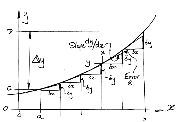
We increase x in small steps, δx, from a to b. For each step we obtain an estimate, δy, of the change in y by multiplying the slope, dy/dx, on the left edge of the step by the width of the step, δx. Our δy is too small by a distance ε because, in our example, dy/dx is increasing with x. But dy/dx is continuous, so as δx→0, the change in the slope across the step becomes negligible, and ε/δy→0. For small enough steps, we can ignore ε. The total change in y from x = a to b is marked as Δy in the diagram. As δx→0, Δy becomes equal to the sum of all the δy = (dy/dx)δx for all the infinitesimal steps δx. We say that Δy is the integral of dy/dx with respect to x from a to b.
The value of f (x) is the derivative of the area under the graph of f (x). If this area A can be described by some function g(x), then g'(x) = f (x). We say that g(x) is the integral of f (x). The act of determining the integral we call integration. Integration is the opposite of differentiation. When f '(x) is the derivative of f (x), then f (x) is the integral of f '(x).
Example: Velocity is the derivative of position with respect to time. If x is the position of an object along a straight line, and t is time, then velocity v = dx/dt. Conversely, the displacement of our object (its change in position) is the integral of its velocity. If we plot v versus t, the displacement between two moments in time is the area under the curve of between these two moments in time. Thus we obtain displacement by integrating velocity.
Example: Suppose our function is f (x) = 2x. What is the area under f (x) from x = 0 to x = 10? We figured out in an earlier exercise that d(x2)/dx = 2x. So the integral of 2x is x2. The area under the curve 2x is x2. From 0 to 10 the area is 102 = 100.
If f (x) is negative, then g'(x) is negative, which means the area under the curve is decreasing. In the regions where f (x) is negative, the area under f (x) is negative also.
Example: The function sin(x) is symmetric about zero in the interval x = 0 to x = 2π. The area under the curve from 0 to π is positive. The area under the curve from π to 2π is negative. The positive and negative areas have equal magnitudes. They add to zero. The total area under sin(x) from 0 to 2π is zero.
The notation below expresses the concept of summing an infinite number of vertical slices each of area f (x) dx, where dx is an infinitesimal change in x.
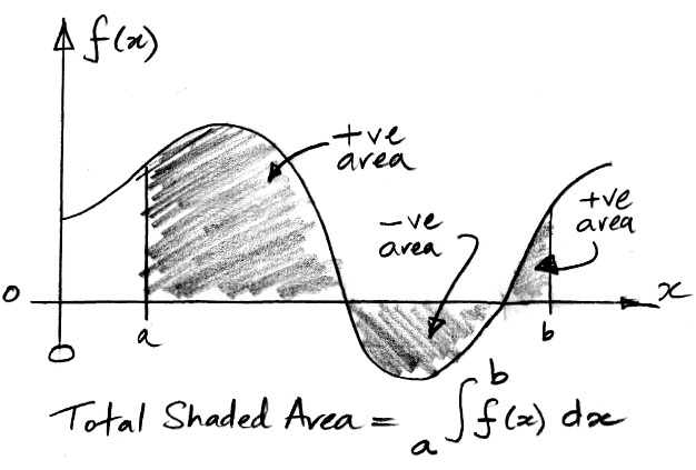
The integral symbols is a stretched letter S for "sum". The sum is from one value of x to another. In the example above, we are summing from x = a to x = b. We call a and b the lower and upper limits of the integration. The term f (x) dx denotes the infinitesimal slices that are to be summed together to obtain the total area. Each slice has finite height f (x) and infinitesimal width dx.
When we say, "the integral of f (x)," we mean, "the integral from zero to x." The lower limit is zero and the upper limit is some unspecified value of x. The integral of 2x is x2. The value of an integral with limits a and b is the value of the integral from 0 to b minus the value of the integral from 0 to a.
Example: What is the area under 2x from x = 4 to x = 5? The area from zero to four is 16, and the area from zero to five is 25, so the area between four and five is 25 − 16 = 9.
As we saw earlier, we have a procedure for determining the derivative of any function. We calculate the change in the function for dx, then divide by dx to obtain the derivative. No such procedure exists for determining the integral of a function. If we know the limits of our integral, we can use numerical integration to obtain a numerical value for our answer. An integral with known limits is called a definite integral. An indefinite integral is one where we do not specify the limits, but instead obtain a formula that gives the integral for all values of x. We cannot obtain the indefinite integral of a function by numerical integration. To obtain the indefinite integral we must either guess the integral and then check our guess, or examine a table of integrals and adapt a similar integral to our problem. We make a table of integrals by differentiating a bunch of functions and tabulating our results. When we see our function in the derivative column, our integral is the function we differentiated.

The derivative of u(x)v(x) is the product rule of differentiation, which we derived earlier. The integral of u(x)v'(x) is the rule of integration by parts, which you can derive from the product rule by noting that the integral of v'(x) is v(x).
The function exp(−x2) appears in the normal distribution. Its integral is the error function, denoted erf(x), which we obtain by numerical integration. The error function is an indefinite integral: we have no formla for it. We can look it up in a table of values, or we can calculate it with a computer. You will find our own error function routine in this library.
Example: What is the derivative of sin2x? We don't have this one in the table. But we do have the derivative of sinax. We can set a = 1. And we have the derivative of f (x)n. We can set n = 2. So let f (x) = sinx. Then d(sin2x)/dx = 2cosx sinx. We could also use the product rule, by letting u(x)v(x) = sinx sinx, and then we have d(sin2x)/dx = cosx sinx + sinx cosx = 2cosx sinx.
Example: What is the integral of sin2x? We use the trigonometric identity sin2x = ½ − ½cos2x. One row of the table tells us the integral of cos2x is ½cos2x. Another row tells us that the integral of 1 is x. The integral of sin2x is: x/2 − sin2x/4.
In the following example, obtain the formula for the area of a circle by integrating the formula for the circumference of a circle. We divide the circle's area, A, into infinitesimal annuli of radius x, and thickness dx. We obtain a formula for the area of each of these infinitesimal annuli. We integrate to this formula from radius zero to the full radius of the circle so as to obtain the total area of the circle.
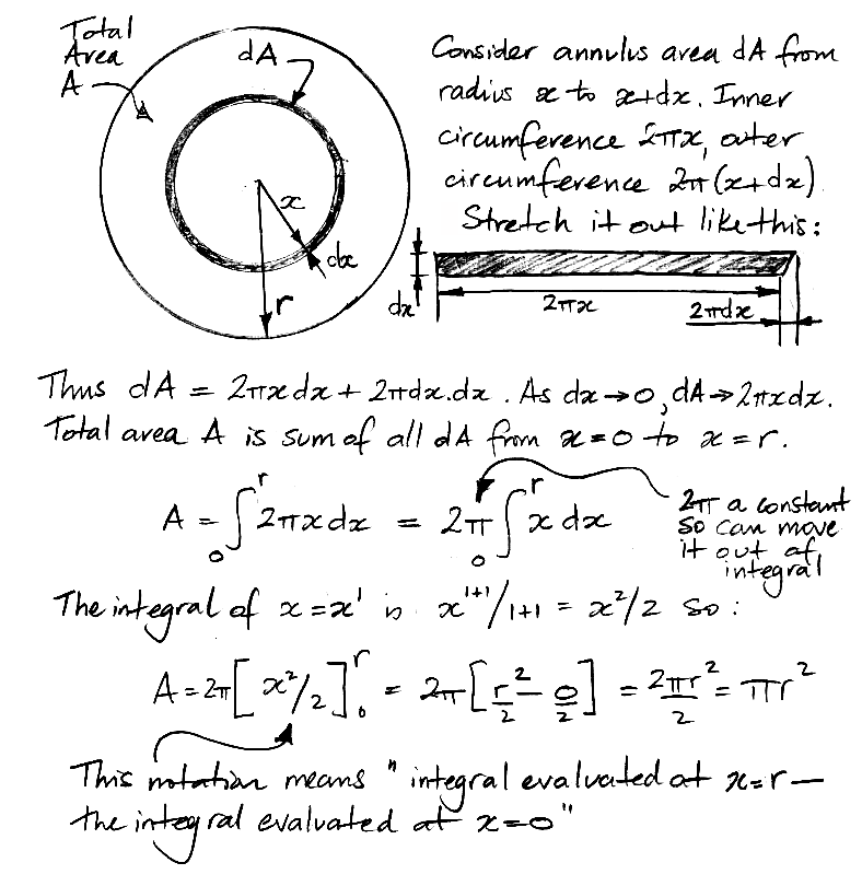
The notation we use at the end of the derivation, with square brackets and the limits of integration on the top-right and bottom-right, is standard notation for a definite integral. We subtract the value of the indefinite integral at the bottom limit from its value at the top limit, and so obtain the definite integral.
Exercise: Consider a circular cone pointed at one end, radius r at the other end, and length l. Obtain the formula for the volume of the cone by integration of the above-derived formula for the area of a circle.
Suppose we have a large number of particles colliding with one another randomly and elastically, constrained within a rigid box. A histogram of the kinetic energy of the particles will have the shape of e−E/kT, where E is kinetic energy, T is absolute temperature, and k is the Boltzmann Constant. The probability density function for kinetic energy is Ce−E/kT for some constant C. The area under a probability density function must be one, so we can determine C by integrating Ce−E/kT from E = 0 to ∞. In the derivation below, we find C for the Boltzmann Distribution, and integrate again to obtain the probability that a particle will have kinetic energy greater than a minimum EJ.
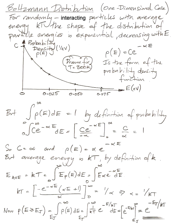
This probability that energy will be greater than a minimum is the Boltzmann Factor.
Some functions of x defy our efforts to obtain an integral function. But if we plot f (x) ourselves, we could measure the integral by dividing the area under the curve into many thin, vertical strips, just like the δA strip in our earlier diagram. Each of these strips would have area f (x)δx. This procedure for finding the integral is called numerical integration. As δx→0, our measurement becomes impractical for a human being, but not for a computer. When all other methods of finding an integral have failed, numerical integration is the method we turn to.
Example: The normal distribution cannot be integrated. But we can obtain its integral by numerical integration. The error function is an example of an integral we can obtain only by numerical methods. It is the integral of a function closely related to the normal distribution function.
In this section, we demonstrate numerical integration using functions for which we can calculate the definite integral. That way, you can check the results of our numerical integration for yourselves.
The average value of sinx is zero for the interval 0 to 2π radians. The average of sin2x is not zero, because the square of both negative and positive values are both positive. The root mean square of sinx is the square root of the average value sin2x from 0 to 2π. The root mean square of a function is measure of how much the function deviates from zero, even when its average value is zero. One way to calculate the mean square of sin2x is to pick a large number of evenly-spaced values of x, calculate the value of sin2x at each of these values of x, and take the average. That's what we do in the SIN2X sheet of Calculus.ods (Open Office spreadsheet), which we invite you to download and examine.
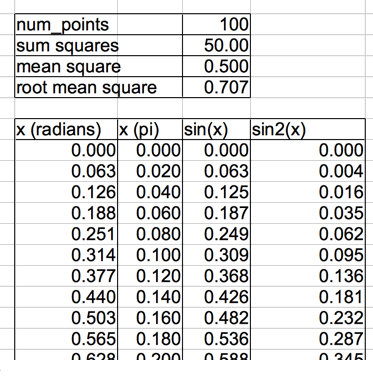
The figure above shows the top rows of the spreadsheet, showing x in units of radians and in multiples of π, sinx, and sin2x at one hundred points from 0 to 2π. There is also a plot of sinx and sin2x, which shows how sin2x is always positive, which we reproduce below.
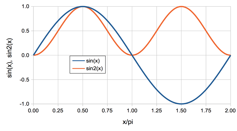
Our values of x start at 0.00π and proceed in steps of 0.02π until we get to 1.98π. We do not continue to 2.00π, because that would be 101 points. Furthermore, we would be repeating our consideration of x = 0.00π, because the value 2.00π begins a new cycle of sinx, where 2.00π is equivalent to 0.00π. Adding these 100 values together, we get a sum of 50.00. We divide by 100 and find that the mean square of sinx is 0.5. The root mean square is 0.707 = 1/√2.
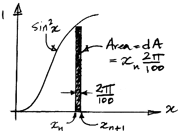
Now consider our spreadsheet calculation this way: we take 100 values of x, and at each value of x we imagine a thin vertical slice of sin2x, of height sin2x and width 0.02π. Its area is 0.02πsin2x. We add the areas of all these slices together to get and estimate of the total area under the graph of sin2x from 0.00π to 2.00π, because the final slice extends to 2.00π. We say an estimate because the top edges of the individual slices always horizontal. They do not follow the continuous line of sin2x. The area of slice number n is 0.02πsin2xn and the sum of all their areas is 0.02π times the sum all 100 values of sin2xn. The length of this area is 2.00π. If we divide the area by 2.00π we the average height of the area, which we see is 0.01 times the sum of 100 values of sin2xn, which is the average value of sin2xn.
Rule: The average value of a function f (x) between x = a and x = b is the integral of f (x) from a to b divided by (b−a).
What we call numerical integration is where we divide the area under a curve into a large number of slices, and we add the slice areas together to obtain an estimate of the total area under the curve, which is an estimate of the integral of the curve. With a large enough number of slices, our estimate can be as accurate as we need it to be. What we did in our spreadsheet is calculate the area under sin2x by numerical integration, and then used the above rule to obtain the average value of sin2x from our estimate of the integral.
Exercise: Calculate the integral of f (x) = x3 + 6x + 5 from x = 0 to 2 by numerical integration using steps of δx = 0.1 and δx = 0.01. Compare your result to the exact integral of f (x) from x = 0 to 2.
Suppose we dig up a 1-g fragment of charcoal from an archaeological site. We want to figure out how old it is using carbon-dating. The concentration of carbon-14 in charcoal made from new wood is one part per trillion = 1 ppt = 10−12, because that's the ratio of carbon-14 to carbon-12 in the atmosphere. Our 1-g piece of charcoal is almost entirely made of carbon-12, so it contains 1/12 mole of carbon-12. If the charcoal were new, one in 1012 of these carbon atoms would be carbon-14. Using Avogadro's constant, the number of carbon-14 atoms in the 1-g fragment when it was first created was 6.0×1023 × 1/12 × 10−12 = 4.2×109 = 4.2 billion carbon-14 atoms. But one in 8000 carbon-14 atoms decays into nitrogen-14 every year, and when they do so, they emit an electron, which we can detect with a suitable instrument. So we can count the rate at which carbon-14 atoms are decaying in our sample. If the sample were new, we would see 520,000 decays per year, or 59 per hour. But we measure only 3.7 decays per hour. How old is our sample? Let us start by writing down what we know about the rate of decay of carbon-14 as a differential equation.
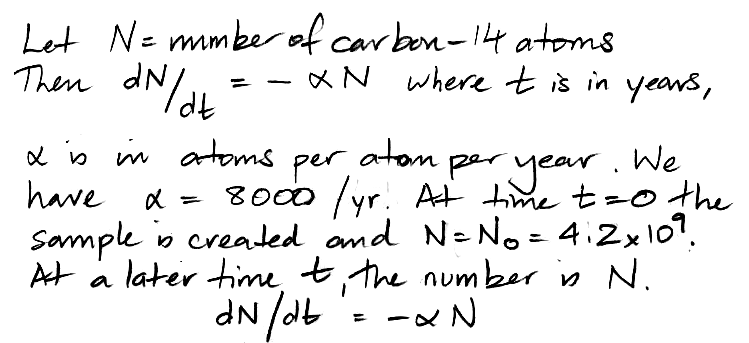
Now we integrate our differential equation to obtain an expression for the number of carbon-14 atoms, N, versus time, t, in years. The notation we use in the following hand-written derivation is similar to the notation we used in the derivation of the area of the circle, but it's not immediately obvious what infinitesimal areas are represented by dN/N and −αdt. The first is the area of a slice of width dN under the graph of 1/N plotted against N. The second is the area of a slice of width dt under the graph of −α plotted against t. The differential equation tells us this: if a change in N of dN occurs in an interval of time dt, then the area dN/N must be equal to the area −αt. We note that dN is going to be negative, because carbon-14 atoms are decaying, while dt is going to be positive, because time is always increasing.
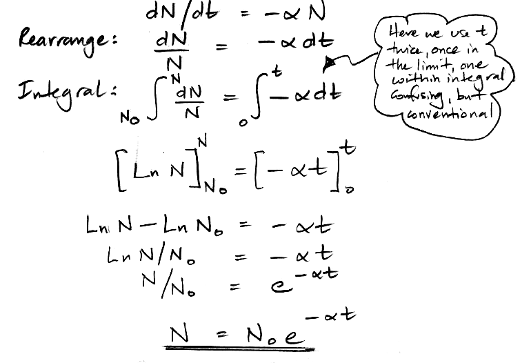
We re-arrange this equation to obtain an expression for the age of the sample as a function of our observed rate of decay. The observed rate of decay is dN/dt, to which we assign the symbol D.

Before we proceed, we check the units of our expression to make sure they are right.

Note that 1/α = 8000 yrs. As another check, try D = 520,000 /yr. We get t = 0 yr. Good. Now, we observe 3.7 decays per hour, or 32,000 decays per year. So our sample is 8000 × Ln(4.2×10⁹ ÷ 8000 ÷ 32,000) = 22,000 yr old.
A differential equation is an equation that equates a function to its derivatives. In the above example, we have the derivative of N with respect to time being equated to the value of N multiplied by a negative constant. Many real-world physical systems are well-described by differential equations. Solving them, we obtain the behavior of these systems with time. As we solve them, we make use of known values of physical constants. In the above example, we knew time started at zero, and that N at time zero was N0. These known values are essential to solving the differential equation, and we call them the boundary conditions of the solution.
When we borrow money from a bank, we pay the bank interest, which is like rent for money. The more money we borrow, the more interest we must pay. As we pay off the loan, the amount of money we still owe the bank is what we call the principle of the loan. The interest rate is the interest we must pay per year for each dollar of principle that remains. If our principle is $100,000 and our interest rate is 3%/yr, we owe $3,000 interest per year. If we pay only $3,000/yr to the bank, we will be paying off only the interest, and the principle will remain $100,000. If we pay $10,000 in the first year, we will pay off $7,000 of the loan, leaving $93,000, and the next year we will owe less interest. Suppose we want to pay off the entire loan in 10 years, making small, frequent payments. What will our total annual payment be?
We need to solve a differential equation to obtain the annual payment. In the following derivation, we imagine that we are paying continuously in infinitesimal amounts for each infinitesimal payment period.
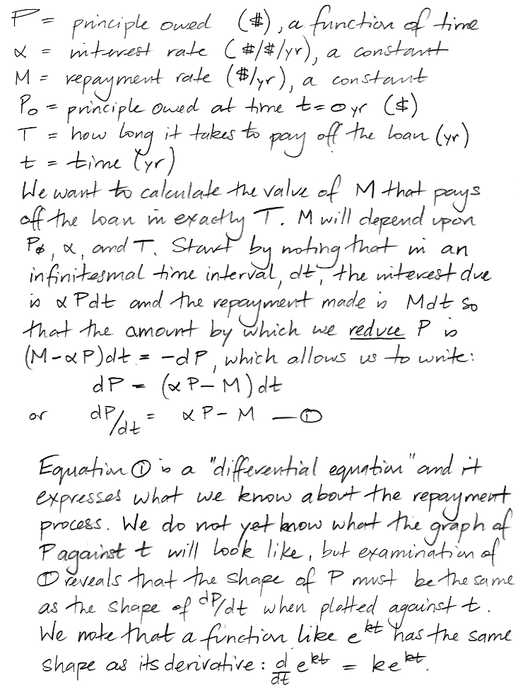
Equation (1) does not tell us the value of P at time t. We assume, however, that there exists some equation that will give us the value of P in terms of t. We now guess what this equation will look like, and then test our guess to see if it satisfies the differential equation. For brevity's sake, our first guess is correct. Any other guess would result in a contradiction when we tested it against Equation (1).
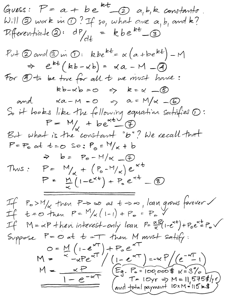
Our value of M is the fixed annual payment rate that repays the entire loan with interest in time T. The time T is the loan term. We divide M into twelve parts to make monthly payments. The following table gives the payment rate for various interest rates, loan terms, and amount borrowed. We also give the total amount paid over the course of the loan.

In the case of a 30-year mortgage at 3%, we end up paying the bank a total of 50% more than the initial loan amount. At 10%, we pay triple the loan amount over thirty years.
Exercise: We throw a ball straight up in the air with velocity 32 m/s. Until it hits the ground again, the ball decelerates at g = 10 m/s/s due to gravity. Let h be its height above the ground. Write down a differential equation relating the second derivative of height to g. Solve the differential equation to obtain h as a function of time, using boundary condition h = 2 m at t = 0. At what time does the ball hit the ground?
Exercise: Obtain the formula for the volume of a sphere of radius r in the following way. Imagine the sphere as a globe upon which we have an equator and lines of latitude. Express latitude in radians, not degrees. Obtain an expression for the surface area of an infinitesimal strip around the sphere that coveres latitude θ to θ+dθ. Obtain the total surface area of the sphere by integrating from −π/2 to +π/2 radians.