 Rasnik Analysis
© 2007-2020, Kevan Hashemi, Brandeis University© 2021-2024, Kevan Hashemi, Open Source Instruments Inc.
[20-MAY-24] A rasnik instrument (Red Alignment System of NIKhef) is an alignment instrument consisting of an infra-red illuminator, a precise chessboard mask, an image sensor, and possibly a lens. In this report we provide a brief introduction to rasnik instruments, but our main focus will be upon the workings of our rasnik image analysis routines. These routines are bundled with our Long-Wire Data Acquisition (LWDAQ) Software, which you can download for free. You can use the routines from the LWDAQ command line, or call them in TclTk scripts, or link them into your own executable.
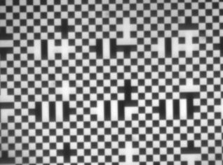
A rasnik mask is a precise, uniform chessboard pattern deposited as a thin aluminum film on a piece of glass. Some of the squares are flipped from black to white, others are flipped from white to black. The flipped squares are code squares. The code squares tell us which part of a rasnik mask we are looking at, even if the mask is much larger than the portion of it we view.
The most common rasnik instrument in our alignment systems consists of a mask, lens, and image sensor. The lens focuses an image of the mask onto the image sensor. Together, these three elements form a three-point monitor. They measure the movement of the center of the lens off the line joining the center of the mask and the center of the image sensor. The mask is a chessboard-like pattern on a piece of glass, illuminated from behind by diffuse light. We can use any kind of image sensor, but we must be sure that we read out each pixel individually, so that our digital image represents exactly the optical image, limited only by the precision of the image sensor pixels themselves.
When the three components of a rasnik three-point monitor move with respect to one another, the mask image moves or changes size on the image sensor. In all rasnik applications, the mask is much larger than the image sensor. The idea is to permit small, inexpensive image sensors to perform alignment measurements over a wide range of positions, as wide a range as is covered by the mask. Typical masks are 30 mm square, but we have masks that are 100 mm square. Our original TC255P image sensors were only 3.4 mm × 2.4 mm. Our newer ICX424AL image sensors are 5.1 mm × 3.8 mm.
When the three components are lined up perfectly, as in our sketch, and the lens is placed so as to give a sharp image like the one we show above, the center of the mask will be focused onto the center of the image sensor. The mask can move almost half its width in any direction, and still cover the image sensor entirely with the mask pattern. The code squares define a two-dimensional coordinate system in the mask, so that any point in the mask has an x and a y coordinate. The purpose of rasnik image analysis is to determine the point in the mask that is focused onto a reference point in the sensor. We most often use the top-left corner of the image sensor as our reference point, because this point is independent of the dimensions of the image sensor. But we can also use the center of the sensor area, or any other point we care to define. The rasnik position is the mask coordinates of the point in the mask that is projected onto the reference point in the image sensor. It consists of two values x and y in microns.
Another way to use a rasnik mask is to press it up close to our image sensor to make a contact print by projecting the mask onto the sensor using light that is perpendicular to the image senor and mask surfaces. Such contact-print rasnik instruments are useful in calibration stands where we want to measure the location of image sensors within a test fixture.
The smallest mask squares we use are 85 μm wide. The largest are 340 μm wide. When the lens is closer or farther from the mask than the image sensor, the mask image will be magnified or demagnified. We choose a mask square size that give us between twenty and thirty squares across the image sensor, so there are plenty of edges for our anlysis to find, and plenty of code squares to decode.
With a sharp image and less than a meter between the mask and image sensor, we can determine the rasnik position with a precision of a tenth of a micron. With sixteen meters between the mask and image sensor, the image becomes blurred by diffraction at the lens, and moves around because of turbulence in air. The precision of a sixteen-meter three-point rasnik is more like ten microns. If you place a rasnik in an evacuated tube, as NIKHEF has done, the rasnik resolution over a hundred meters is less than a micron.
For an explanation of the rasnik from its creators, see the Rasnik Home Page. For our published paper on Rasnik three-point monitors see The Rasnik 3-point optical alignment system. The table below presents further docoments.
| Title with Link | Description |
|---|---|
| ATLAS Encap Alignment | Description of several practical rasnik instruments. |
| Depth of Field | How to balance focus and diffraction to maximize depth of field. |
| LWDAQ User Manual | Long-Wire Data Acquisition hardware and software manual. |
| Rasnik Instrument Software | Our rasnik instrument graphical user interface. |
| Image Analysis Software | Source code of our analysis library, compile with FPC. |
| Steepest Ascent Algorithm | Our original, now obsolete, rasnik analysis. |
| Pixel CCD RASNIK | Original rasnik instrument image sensors. |
| Pixel CCD RASNIK DAQ | Oiginal data acquisition system. |
We first began working with rasnik instruments at Brandeis University in 1997. Some of the documents in the table above date from that time.
[20-MAY-24] Our LWDAQ Software is available as a GitHub repository and as a zipfile download. The software runs on MacOS, Linux, and Windows. Installation instructions are here. Open LWDAQ and select the Rasnik Instrument from the Instrument Menu. Press Read and select one of the example images in the Images library. The rasnik analysis will find the rasnik pattern, determine the rasnik position, rotation, magnification, skew, and slant. It will mark the pattern it finds on the images.
Press the Info in the instrument panel to open the Info Panel. There you can set analysis_show_fitting to "1000". Press Acquire again. You will see the analysis pausing for one second at a time, and at each pause, you will see a different stage of the rasnik analysis. Set analysis_show_fitting to "-1" and the analysis will pause at each stage until you press a button. By default, the Rasnik Instrument produces a single line of numbers like this:
Rasnik_benchmark.gif 32535.26 24236.77 0.469865 0.470965 8.519 0.554 120.0 10.0 4 1720.0 1220.0 0.464 0.019 1.140
The more verbose result from the same instrument looks like the print-out below, and includes a description of each parameter. The exact numbers are not the same as above because we acquired a second image and analyzed it to obtain the output.
Rasnik_benchmark.gif
Mask Position X (um in mask coordinates): 32535.26
Mask Position Y (um in mask coordinates): 24236.77
Image Magnification X (mm/mm): 0.469865
Image Magnification Y (mm/mm): 0.470965
Image Rotation (mrad anticlockwise): 8.519
Measurement Precision (um in mask): 0.554
Mask Square Size (um): 120.0
Pixel Size (um): 10.0
Orientation Code (the code chosen by analysis): 4
Reference Point X (um from left edge of CCD): 1720.0
Reference Point Y (um from top edge of CCD): 1220.0
Image Skew X (mrad/mm): 0.463
Image Skew Y (mrad/mm): 0.019
Image Slant (mrad): 1.140
For an explanation of the reference and orientation codes, see here. The reference code determines the reference point on the image sensor. When we compare rasnik analysis programs, our tradition is to use the top-left corner of the top-left pixel as the reference point, because this point is easy to define when we have images of varying sizes. It's the top-left corner of pixel (0,0).
A rasnik measurement is the determination of the point in the mask that is projected onto the reference point in the image sensor. It may be that the reference point is not a light-sensitive pixel. It may be part of a black left-hand border in the image. But we can still calculate which point in the mask would have been projected onto the reference point if the reference point were a light-sensitive pixel. The rasnik measurement consists of the x and y coordinates of a point in the mask, the magnification of the mask image, and the rotation of the mask with respect to the image sensor.
[20-MAY-24] Our LWDAQ Sources directory contains our analysis code, which is written entirely in Pascal. We compile all our analysis libraries with the Free Pascal Compiler (FPC) by typing "make" in the Build directory. The build produces a 64-bit ".dylib" for MacOS, ".dll" for Windows, and ".so" for Linux and Raspbian. You can call our rasnik analysis from the LWDAQ console using the lwdaq_rasnik command. You will find a description of this and every other LWDAQ command in our Command Reference. The lwdaq_rasnik routine is declared in lwdaq.pas. The lwdaq_rasnik routine calls many other procedures named rasnik. These are to be found in rasnik.pas. At the bottom of lwdaq.pas you will see where lwdaq_rasnik is installed into LWDAQ's TCL command interpreter. You can load our dynamic library into your own Tcl application. Or you can make analysis to create a static library that you can link to your own compiled code.
[20-MAY-24] We pay close attention to the routine's execution time, which we can obtain at any time using the Rasnik Instruments analysi_show_timing parameter. Open the Info panel, find this parameter, and set it to one. Now analyze Rasnik_benchmark.gif, which is available in the LWDAQ Images directory. We obtain the following output on our 1.1 GHz, 64-Bit, 2020, Intel MacBook Air running LWDAQ 10.6.10.
Index, Elapsed (ms), Comment:
     0      0 beginning rasnik analysis in lwdaq_rasnik
     1      0 generating image derivatives in lwdaq_rasnik
     2      2 clearing overlay in lwdaq_rasnik
     3      3 starting rasnik_find_pattern in lwdaq_rasnik
     4      4 starting rasnik_refine_pattern in lwdaq_rasnik
     5     16 starting rasnik_adjust_pattern_parity in lwdaq_rasnik
     6     16 starting rasnik_identify_pattern_squares in lwdaq_rasnik
     7     19 starting rasnik_identify_code_squares in lwdaq_rasnik
     8     20 starting rasnik_analyze_code in lwdaq_rasnik
     9     23 starting rasnik_from_pattern in lwdaq_rasnik
    10     23 starting rasnik_display_pattern in lwdaq_rasnik
    11     25 starting to dispose pointers in lwdaq_rasnik
    12     25 done in lwdaq_rasnik
We find that execution time is pretty much inversely proportional to clock speed on all modern computers. The rasnik analysis will occupy one processor core full-time until it is done, so having two cores while analyzing many rasnik images will help. Laptops can boost their clock speed briefly to provide rapid analysis, but if they are required to analyze a large number of images, they will slow down to avoid over-heating.
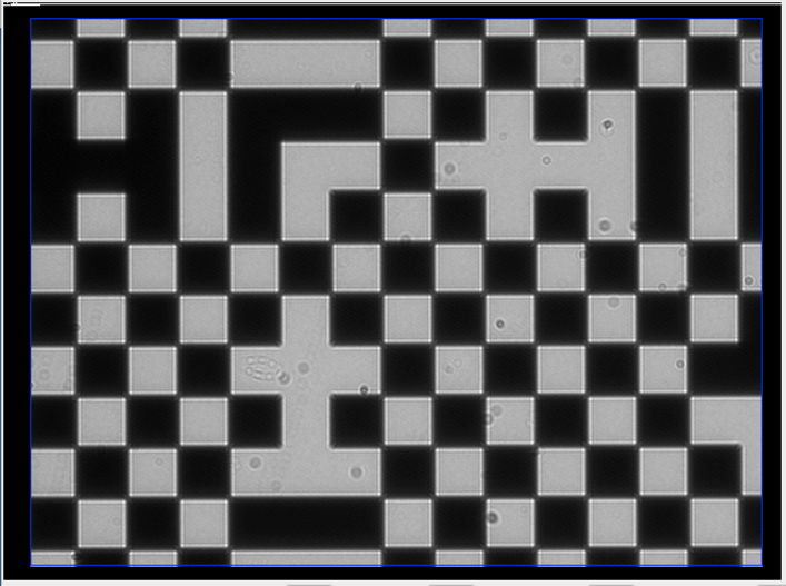
[20-MAY-24] We use two derivative images to find the chessboard pattern. One contains the absolute value of the horizontal intensity derivative, and the other contains the absolute value of the vertical intensity derivative. The image below shows the horizontal derivative image of the same rasnik image we present in our Introduction.
Notice how both the left and right edges of each square appear as white lines in the derivative image. A dark-to-light transition has the same appearance in the absolute-value derivative as a light-to-dark transition. It is this absolute value that allows us to find the edges in the chessboard pattern, because in the absolute-value derivative, the edges are continuous and bright.
The routines for calculating derivative images are image_grad_i and image_grad_j, defined in image_manip.pas. The image structure itself is defined in images.pas.
[31-MAY-24] Once we have the derivative images, we use them to determine the period and phase of the chessboard pattern. We take a strip along the top of the horizontal derivative image and calculate its vertical intensity profile by summing the intensity of the pixels in each of its columns. We calculate the spatial frequency spectrum of this profile using a discrete fourier transform. To improve the performance of the fourier transform, we first subject the vertical intensity profile to a window function. When our original image contains a chessboard pattern, the largest component in the spectrum will correspond to the spatial frequency of the chessboard squares. The phase of this component corresponds to the position of the first chessboard edge from the left side of the image.
Fourier analysis of intensity-profiles takes place in rasnik_find_pattern, which calls profile_by_fourier. The profile_by_fourier routine makes a single call to fft_real, which is defined in utils.pas. The fft_real function is a fast Fourier transform that insists that the number of samples be an exact power of two. If we have 320 points in our profile, we pass to the fast fourier transform these 320 points along with another 192 points whose value we set equal to the average value of the first 320. These 512 points give us 256 discrete frequency components in the transform. Each frequency is a multiple of the fundamental frequency represented by a strip 512 columnes wide. The first term in the spectrum is the zero frequency term, or average intensity. The second term has period 512 columns. The last has period two columns.
Example: Suppose we have squares that are roughly four pixels high, and we use 256 rows for our fourier transform. Our spectrum contains components with the following periods close to four pixels: 3.46, 3.51, 3.56, 3.66, 3.71, 3.76, 3.82, 3.88, 3.94, 4.00, 4.06, 4.13, 4.20, 4.27, 4.34, 4.41. The estimate we obtain from our fourier transform will be within 1% of the correct period.
Here is the fourier spectrum we obtain for a strip 30 pixels high along the top of the horizontal derivative of three of our sample images. We plot the amplitude of the components versus the period in pixels, as opposed to versus frequency in 1/pixels. You will find these images in our LWDAQ/Images directory.
Each spectrum has a peak intensity that stands out from the rest of the spectrum. If we consider the ratio of the peak amplitude to the average amplitude, we obtain a simple criteria for rejecting images that contain no periodic pattern. The peak ratio for a sharp rasnik image is between 20 and 40. For a blurred image with nine squares across, the ratio is still 10. When we reduce the exposure time until we can barely see any sign of the pattern, even with image intensification, the peak ratio drops to 3.0. Noisy or blank images, however, have peak ratios less than 2.0. We choose 3.0 as our threshold for acceptance. The rejection is set by min_peak_ratio in the profile_by_fourier routine.
The following image, Rasnik_dim.gif, has peak to average ratio of 5.0. We use exact intensification in the Rasnik Instrument to see the rasnik pattern, which would otherwise be invisible. We acquired Rasnik_dim.gif with a 200-μs exposure time.
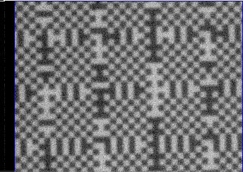
The period and phase of the largest component in the spectrum are a good estimate of the size and offset of the chessboard pattern. But the discrete jumps from one frequency to the next in the spectrum prevent us from obtaining a more accurate measure of the period with the fourier transform. If possible, therefore, we try to refine our measurement of period and offset by taking a closer look at the profile, knowing ahead of time the approximate size of the squares.
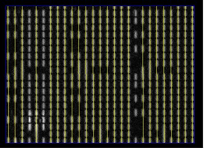
The Fourier transform will sometimes pick the second harmonic of the square pattern rather than the fundamental, which causes analysis to fail. We encounter this problem with contact print images of rasnik masks, where we press the mask up against our image sensor window and project the mask pattern with collimated light.
The Fourier transform routine that makes the first estimate of the square size chooses the second harmonic of the square pattern instead of the fundamental. The black squares are larger than the white squares. The edges of the white squares contain interference fringes. The gradient image consists of thin lines. The second harmonic exceeds the amplitude of the first.
We can analyze the above image perfectly well, and quickly, by using a pre-filter. We shrink the image by ×3 or ×4 and we obtain an accurate and rapid analysis result.
[20-MAY-24] The fourier analysis of our derivative image gives us the spatial period of the mask pattern to within 1% when the square are 4 pixels across. If we have eighty squares across our image, this 1% error in spatial frequency will cause our estimate of the locations of the peripheral pattern edges to be misplaced by up to 1% * 80 / 2 = 40% of a square width. That's not good enough. Our objective in analyzing the image slices is to isolate one edge from another so that we can fit lines to the edge pixels and obtain the edge locations with as much accuracy as possible. Before we can do that, we need to be sure that we know where the edges are to within at least 10% of a square width.
To improve our measurement of square size and offset we use a method of smoothed peaks. Using approximate knwoledge of the square size, we create a spatial band-pass filter and apply it to our intensity profile. We do this for every slice down to the bottom of the image. In each slice, we try to determine the square size from the locations of the maxima in the filtered profile. The number of slices we analyse in each direction on the image is given by rasnik_num_slices. The more slices, the greater the mask rotation we can accommodate. The smoothed peak routine is profile_by_maxima, called from rasnik_find_pattern, both in rasnik.pas. Whenever the filtered profile fails to give us a good estimate of the period and offset, we revert to the estimate provided by a fast fourier transform of the slice.
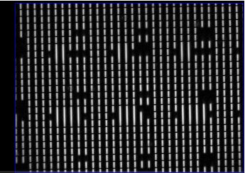
The spatial band-pass filter gives us peaks that correspond to edges in the pattern. Some edges do not appear as maxima because the edges do not appear in the slice. The following image shows the horizontal band-pass filtered profiles for eight slices.
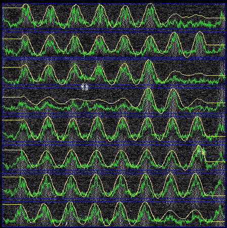
In some slices we see that peaks are missing or obscured. Code squares disrupt the regularity of the chessboard in the slices. Nevertheless, we almost always overcome these irregularities, and we use the peaks to obtain a better estimate of the pattern frequency, rotation, and offset. We call the resulting estimate our approximate pattern. If one of the slices fails to provide a useful sequence of maxima, we calculate the fourier transform of the profile and use the period and phase of the largest component instead. In that case, the filtered profile will be red in a plot like the one we show above.
[20-MAY-24] Our approximate pattern is good to a few microns in position, but only 1000 ppm in magnification. We would like our magnification accuracy to approach 10 ppm. So we go on to refine the fit further. The approximate pattern is good enough to allow us to isolate edges in the derivative images. Given any bright pixel in the derivative image, we can tell which edge it corresponds to, and add it to a straight-line fit that will tell us with better accuracy where the edge is.
We divide the derivative image into strips parallel to the vertical edges, and fit straight lines to the pixels in each strip. We weight each pixel by its intensity so as to favor brighter edge pixels. Nevertheless, noise pixels far from the line can displace the fit significantly. We consider the slope and offset of all the lines and reject any that are more than two standard deviations from the mean obtained from the entire set. The straight-line fitting is done in rasnik_refine_pattern, which takes as input not only the horizontal and vertical derivative images, but also the approximate pattern obtained by rasnik_find_pattern.
The following figure shows the lines we fitted and used in our analysis of a sharp rasnik image. We see that even in a good image, we reject some of the lines, and these tend to be ones most distrupted by dirt or code squares.
When the magnification of the mask changes with position in the image, we say the image has skew. The change in magnification from left to right is the x-direction skew, and from top to bottom is the y-direction skew. We measure the x-skew by looking at how the slope of the horizontal lines changes from top to bottom in the image. We express the skew in units of mrad/mm. When the x-skew is positive, the horizontal lines are diverging from left to right. The y-skew we obtain from the variation in the slope of the vertical lines from left to right. When the y-skew is positive, the vertical lines are diverging from top to bottom. In a skewed image, the pattern x and y-directions are not everywhere perpendicular in the image. If they are perpendicular at the center of the analysis bounds, where our analysis places the origin of the pattern coordinate system, then the x and y skew parameters are sufficient to describe the skewed image, including correct orientation of the pattern coordinates in other parts of the image where they are not perpendicular. But if the pattern coordinates are not perpendicular at the center of the analysis bounds, we must account for this non-perpendicularity with another rasnik parameter: the image slant. The slant is the angle by which the pattern coordinates are less than perpendicular at the pattern origin.
[20-MAY-24] Now that we have the frequency, rotation, and offset of the chessboard-like mask pattern, we need to set the parity of the pattern, which is to say: we need to know which squares are nominally white, and which are nominally black. Code squares are squares that are out of parity. The critical operation in determining the parity of the pattern, and then the parity of individual squares with respect to the pattern, is determining whether or not each square is black or white. Because the intensity of the mask illumination can vary across the mask, we cannot rely upon comparing each square to an average intensity. Nor can we take a single pixel from a square and compare it to a single pixel in neighboring squares. Dust and noise in the image will defeat any judgment that uses single pixels.
The square_whiteness routine is in rasnik.pas returns the whiteness of a square. The rasnik_identify_code_squares routine decides which squares are code squares and which are not, by comparing its center intensity to the center intensity of its neighbors. We calculate the center intensity of each square in one pass through the pattern array with rasnik_identify_pattern_squares.
We must determine if a variation between one square and the next is significant. We use the standard deviation of intensity as our measure of significant variation. We compare the amount by which a square is whiter than its neighbors to the standard deviation of the image intensity, and so decide if the difference is significant. The image_amplitude routine is in images.pas. This routine is not deterministic: it determines the amplitude of an image by looking at ten thousand randomly-selected pixels. But it is several times faster than a routine that looks at all points in a typical image, which might contain four hundred thousand pixels. You can see this non-determinism sometimes, when a dim image has a piece of dirt that almost turns a white square into a black square. Sometimes the routine decides the square is a code square, and sometimes not. This is because of tiny variations in the result of image_amplitude.
Identifying the code squares requires that we determine the center intensity of each square, and compare it to the center intensity of its neighbors. Once we identify the code squares, we try to interpret them. This endeavor is greatly complicated by the fact that there may be many false code squares in the image, and by the fact that we may not know the orientation of the mask pattern. On the other hand, correct code squares are severely constrained in the way they relate to one another. By checking the available code squares against the constraints of an uncorrupted rasnik pattern, we can reject erroneous code squares, determine the correct rotation of the mask, and so arrive at an accurate and reliable measurement. The code analysis is based in rasnik_analyze_code, in rasnik.pas. This routine calls analyze_orientation, in which you will find the bluk of the code-square interpretation and checking.
The analyze_orientation routine assumes a particular mask orientation and goes through all the canditate pivot squares in the image calculating their x- and y-direction code values from adjacent code squares. It then looks for sets of pivot squares whose x- and y-codes agree. It assigns a score to the orientation, which is the number of pivot squares in the largest set of pivot squares that agree with one another.
In dim and dirty images, we can get a large number of candidate pivot squares, and these can form several mutually-agreeing sets of the same size. We reject an orientation under such circumstances, by setting the orientation score to zero. We check to see if the number of acceptable pivot squares is above a certain fraction of the available pivot squares. In this way, we reject an orientation if there are too many unacceptable pivot squares. We also check to see if all acceptable pivot squares are separated by an integer multiple of code_line_spacing squares in both the x- and y-directions.
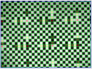
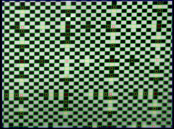
When it's finished anlyzing the code squares, the analysis routine draws its results on top of the image, as you can see here. It marks pattern edges with green lines and code squares with little rectangles. The rectangles are red if the code square lies at the intersection of two valid binary code numbers. We call the red squares pivot squares. The rectangles are yellow if the code square is not a pivot square. If you have show_fitting set when you call the analysis, you will see all the remaining, usable squares in the image marked with a blue rectangle. The display makes it easy for us to identify the cause of analysis failure, and has been of great help to us in our efforts to improve and accelerate the analysis.
[20-MAY-24] When we pass a non-rasnik image to the analysis, we want to get an error message as a result, not a rasnik measurement. We use the fourier transform stage of analysis to reject blank or exceedingly distorted rasnik image. Earlier versions of the code relied upon examination of the code squares. These earlier versions would occasionally produce a result like the one shown below.
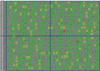
When we obtain an apparantly valid rasnik measurement from a non-rasnik image, we call it a false positive. The false positive rate with noise images like the one shown above is less than 0.01% for LWDAQ 10.6.10+. Rapid rejection of invalid images greatly accelerates our use of random boundries, which we describe in the next section.
[20-MAY-24] When a significant portion of a rasnik image is obscured or distorted by obsticles or dirt, we must find analysis boundaries that enclose the intact portion of the image before we can expect successful analysis. The Rasnik Instrument in our LWDAQ Software will select suitable analysis boundaries automatically after analysis failure if we instruct it to do so. Our Pascal libraries do not perform this selection. Instead, we implement a simple random try-out algorithm in the Tcl. The LWDAQ_analysis_Rasnik routine generates analysis boundaries at random and applies rasnik analysis to the image. It continues trying random boundaries until the analysis succeeds or it reaches its maximum permitted number of attempts. We describe how to set up the random analysis boundary selection in the Rasnik Instrument section of the LWDAQ User Manual.
When we use random boundaries, we will lose measurement accuracy because we are not using all available squares. If we are using the center of the image sensor as a reference point, different analysis boundaries give different mask rotations, and these rotations are multiplied by the distance from the analysis boundary center to the image sensor center when we calculate the point in the mask that is projected onto our reference point.
The graph above shows how x and y position vary as we use a 100-pixel high subset of the analysis bounds drawn on Rasnik_benchmark.gif. We move our subset down from the top of the right side of this image to the bottom. At each step, our bounds cover the full width of the image, but less than half the height. The change in x as we move our bounds downwards is less than half the change in y.
We obtained the above results with the following Toolmaker script, which you can use yourself to obtain similar plots from your own images. Cut and paste the above code into the Toolmaker window and press Execute.
set fn [LWDAQ_get_file_name]
set r [LWDAQ_read_image_file $fn]
set c [lwdaq_image_characteristics $r]
scan $c %u%u%u%u left top right bottom
set height 100
for {set a $top} {$a <= [expr $bottom - $height]} {incr a} {
  lwdaq_image_manipulate $r none -left $left -right $right \
    -top $a -bottom [expr $a + $height]
  set result [lwdaq_rasnik $r \
    -square_size_um 120 \
    -pixel_size_um 10 \
    -reference_x_um 1720.0 \
    -reference_y_um 1220.0 ]
  LWDAQ_print $t "$a $result"
  LWDAQ_support
}
[20-MAY-24] The Rasnik Instrument allows us to smooth and shrink images before analysis. We call these manipulations pre-filtering. When analysis fails on a dim image, it might succeed if we apply smoothing before analysis. If the squares in our image are large, we can shrink the image by a factor of two, three, or four and still find the pattern. Shrinking the image before analysis reduces execution time. It also permits analysis of certain images on the extremes of sharpness: those that are blurred in the extreme and those that are sharp in the extreme. The Rasnik Instrument allows us to introduce pre-filtering through its analysis_enable parameter. The table below gives the rasnik measurement we obtain from Rasnik_large.gif, an image upon which analysis fails in the absence of pre-filtering.
| Code | Pre-Filtering | Result | Time (ms) |
|---|---|---|---|
| 1 | none | Analysis Fails | 15 |
| 11 | smooth | 197715.17 219994.14 1.060788 1.057097 9.688 | 46 |
| 21 | shrink ×2, smooth | 197713.17 219993.68 1.061092 1.053085 10.627 | 23 |
| 31 | shrink ×3, smooth | 197713.36 219989.27 1.062162 1.051370 10.548 | 13 |
| 41 | shrink ×4, smooth | 197716.23 219986.80 1.060502 1.045541 9.876 | 9 |
The x and y measurements vary by less than ±2μm as we smooth and shrink the image. The magnification varies by around 0.2%. Shrinking the image does not make things significantly worse, but it decreases execution time dramatically, and sometimes it makes analysis possible. Our Rasnik_contact library image, for example, is one that requires shrinking by ×3 or ×4 for analysis to succeed.
[20-MAY-24] Our rasnik analysis produces an estimate of its own measurement precision. The error field in our result, which we call the mask error, is the uncertainty in the x and y fields. A rasnik measurement gives us the point in the mask that is projected onto a reference point in the image sensor. The mask error applies to the measured point in the mask, not to the reference point in the image. Nevertheless, our choice of reference point affects the mask error.
Our Rasnik Instrument supports several standard reference points and also custom reference points through its analysis_reference_code, analysis_reference_x_um, and analysis_reference_x_um parameters. The most accurate reference point is the center of the analysis bounds. But this point is not practical in conjunction with random boundaries.
The reference code parameter tells the Rasnik Instrument how to choose the reference point for analysis. The analysis result will be the coordinates of the point in the mask that is projected onto the reference point. Here are the values of reference code defined in Rasnik.tcl.
rasnik_reference_top_left_corner=0;
rasnik_reference_center_analysis_bounds=1;
rasnik_reference_center_ccd=2;
rasnik_reference_image_point=3;
The reference point is a point in image coordinates, and is given in units of micrometers. The image coordinate origin is in the top-left corner of the image. The x-axis runs left to right and the y-axis runs top to bottom. If we use reference code 3, the Rasnik Instrument will use reference_x_um and reference_y_um to specify the reference point. The other reference codes tell the Rasnik Instrument to ignore reference_x_um and reference_y_um, and instead calculate the reference point itself. In the ATLAS end-cap we use the center of the image sensor as our reference point with reference code 2. When we compare different rasnik analysis routines, we use the top-left corner of the top-left pixel with reference code 0.
The center of the images we obtain from our TC255P sensors in the ATLAS end-cap alignment system is (1720 μm, 1220 μm) in image coordinates. For the ICX424 and ICX424Q the center is (2590 μm, 1924 μm).
To calculate the mask error, we start with our estimate of the error in measuring the position of the rasnik pattern at the center of the analysis bounds in the image. We obtain this estimate by looking at the standard deviation of the residuals from the multiple straight-line fits we perform to refine our rasnik pattern. We divide the standard deviation of the residuals by the square root of the number of edge pixels we used. We call this error at the center of the analysis bounds on the image the center point error. We estimate the rotation error by taking the center point error and dividing by the width of the analysis bounds. We multiply the rotation error by the distance from the center of the analysis bounds to the reference point, wherever it may be. This gives us an additional error that we add in quadrature to the center point error to obtain our estimate of the error at the reference point.
where Er is the reference point error, Ec is the center point error, r is the distance from the center of the analysis bounds to the reference point, w is the width of the analysis bounds, and ⊕ is the act of adding in quadrature. We divide the reference point error by the magnification to obtain the mask point error.
As we mentioned above, we estimate our rotation error by dividing the center point error by the width of the analysis bounds (Ec/w). But our rasnik analysis provides us with only the mask error. We can convert the mask error into the reference point error by multiplying by the magnification. We could use the above equation to calculate the center point error from the reference point error, but doing so would require that we knew w and r, the width and center of the analysis bounds with which the rasnik analysis was performed. In general, we don't know these things when we look up an old rasnik result.
We recommend that you estimate rotation and magnification error by dividing the reference point error by the image width. This calculation won't be far wrong when you have analysis bounds that take up more than half the image, but for smaller boundaries, you will under-estimate the error.
Example: We analyze Rasnik_small_bounds, which uses a small analysis boundary in the lower-right of the image. We obtain a mask error 0.8 μm at the center of the analysis bounds (2965 μm, 1965 μm), 1.2 μm at the center of the image (1720 μm, 1220 μm), and 2.3 μm at the top-left corner of the image (0 μm, 0 μm). The magnification is 0.8, so our reference point error in these three cases is 0.64 μm, 1 μm, and 1.8 μm respectively. If we divide by the image width of 3400 μm, we obtain rotation errors 230 μrad, 300 μrad, and 680 μrad. The magnification error will be similar.
As you can see in the example, our rule of thumb leads to differing rotation and magnification errors for the different reference points. But the choice of reference point should not affect either error estimate. Only the position error is affected by reference point. But when we use larger boundaries, our rule of thumb works rather better.
Example: We analyze Rasnik_small_bounds, but with bounds that fill the entire image. We obtain a mask errors 0.09 μm, 0.09 μm, and 0.10 μm respectively. When we divide by the image width we get rotation error 30 μrad and magnification error 30 ppm.
The best images give us a magnification uncertainty of around 30 ppm. When we analyze simulated images, our magnification precision can be as low as 10 ppm, but we have systematic errors much larger than our precision, as we describe in Simulated Images.
[31-MAY-24] One way to test our rasnik anslysis is with simulated rasnik images whose position, rotation, and magnification we know exactly. In rasnik.pas we define a procedure called rasnik_simulated_image. This procedure draws a rasnik pattern in an image. We call this routine from our LWDAQ command line with lwdaq_image_manipulate with the rasnik manipulation. We can specify the location of the top-left corner of a black square in image coordinates, the width and height of the squares in pattern coordinates, the rotation of the pattern, and the sharpness of its intensity variation. The simulated images contain no code squares.
We use the following Toolmaker script to generate simulated images and analyze them. The script generates images with rotation −150 mrad to 150 mrad in steps of 10 mrad. Each image has white intensity noise added, of peak-to-peak amplitude one count.
lwdaq_image_create -width 400 -height 400 -name sim
catch {image delete p}
image create photo p
destroy $f.i
label $f.i -image p
pack $f.i
for {set rot -150.0} {$rot <= +150.0} {set rot [expr $rot + 10.0]} {
  LWDAQ_print -nonewline $t "[format %.1f $rot] "
  foreach s {0.02 0.1 1.0 10.0} {
    lwdaq_image_manipulate sim rasnik "200.0 200.0 20.0 20.0 $rot $s 1.0"
    set result [lwdaq_rasnik sim -pattern_only 1]
    LWDAQ_print -nonewline $t "[format %.6f [lindex $result 2]] "
    lwdaq_draw sim p -intensify exact
    LWDAQ_update
    if {![winfo exists $t]} {break}
  }
  LWDAQ_print $t
}
We place the top-left corner of a black square at location (200, 200) in image coordinates, which places the square 200 pixels to the right of the top-left corner of the top-left pixel and 200 pixels below. The squares are 20 pixels wide and 20 pixels high. For each rotation, we vary sharpness from 0.02 to 10. We display the with our exact intensification, which means that the brightest pixel appears white and the dimmest pixel appears black. At sharpness=0.02 the image intensity is sinusoidal with amplitude 2% of full scale. At sharpness=0.1 the amplitude is 10% and at sharpness=1 the amplitude is 100%. These two images look the same with exact intensification. At sharpness=10, the sinusoid is amplified by 10 and clipped to the black and white levels to give a near-perfect chessboard pattern. Analysis fails on images with sharpness=0.01 or less. Quantization is a non-linear process that creates a double-frequency signal. In the derivative of an image with peak-to-peak amplitude 2 counts, the double-frequency component is larger than the fundamental, as you can see here.
The Toolmaker script applies partial rasnik analysis using the -pattern_only option in lwdaq_rasnik. We measure the location and square size of the pattern. The following graph shows how our magnification varies with rotation for the four different values of sharpness.
Our magnification resolution is roughly 200 ppm for rotations ±100 mrad, but degrades rapidly for greater angles. We obtained plots in the same format for the measured position and rotation. Our position accuracy over the full range of rotation and sharpness is better than 1% of a pixel. Our rotation resolution is around 50 μrad for sharpness ≥0.02.
The following Toolmaker script uses simulated images to test the x-direction measurement of the analysis. Instead of rotating the images we displace them in 0.02-pixel steps and compare the simulated image position with the measured position.
lwdaq_image_create -width 400 -height 400 -name sim
catch {image delete p}
image create photo p
destroy $f.i
label $f.i -image p
pack $f.i
for {set x 202.0} {$x <= 207.0} {set x [expr $x + 0.02]} {
  LWDAQ_print -nonewline $t "[format %.2f [expr fmod($x,10)]] "
  foreach s {0.02 0.1 1.0 10.0} {
    lwdaq_image_manipulate sim rasnik "$x 200.0 20.0 20.0 0.0 $s 1.0"
    set result [lwdaq_rasnik sim -pattern_only 1]
    set rx [expr fmod([lindex $result 0],10)]
    LWDAQ_print -nonewline $t "[format %.2f $rx] "
    lwdaq_draw sim p -intensify exact
    LWDAQ_update
    if {![winfo exists $t]} {break}
  }
  LWDAQ_print $t
}
Our image simulation provides for the inclusion of white noise and we add noise of peak-to-peak amplitude one count to all our images. Thus the images are more like those we obtain from our cameras. We obtain the following graphs of the measurement error for our four values of sharpness. The graph shows systematic errors with period one pixel that get less severe as the image becomes sharper.
The average position error is −0.038, 0.000, 0.000, and 0.000 pixels with increasing sharpness. The standard deviation of the error is 0.17, 0.09, 0.07, and 0.01 pixels with increasing sharpness.
[31-MAY-24] The following constants in our code put limits on the square patterns it can analyze successfully. For a throughh explanation of the function of each constant, see rasnik.pas. These constants can be altered only by editing the source code and re-compiling. We summarize their functions below.
rasnik_min_squares_across=8; {squares}
rasnik_max_squares_across=200; {squares}
rasnik_min_pixels_per_square=2.5; {pixels}
rasnik_num_slices=8;
The analysis will fail on any image in which there are fewer than rasnik_min_squares_across from left to right or from top to bottom of the analysis bounds. It will fail if there are more than rasnik_max_squares_across squares from left to right or top to bottom. It will fail if the squares are less than rasnik_min_pixels_per_square pixels wide or high.
If we reduce the minimum square size to two pixels, the analysis is fooled by blank or dark images. A two-pixel square gives a two-pixel periodic pattern in the derivative image. It is not possible for us to obtain the phase of such a pattern with accuracy better than 180°, so there is not point in attempting to analyze such a pattern. With a two-pixel minimum size, our analysis is fooled by our BCAM_250cm sample image into seeing an array of 100×100 two-pixel squares, resulting in a futile ten-second attempt to find a pivot square.
The rasnik_num_slices constant tells us how many slices the analysis takes across the image in order to obtain the pattern rotation. With eight slices, the routine divides the image from top to bottom into eight equal slices, each of them as wide as the analysis bounds. Each slice provides square edge locations. So long as the edges in adjacent slices line up to within less than half a square width, the pattern rotation will be unambiguous to the routine. Thus rasnik_num_slices determines the maximum acceptaebl rotation of the pattern, which is half a square per slice. With eight slices, the pattern can shift by four squares from top to bottom and four squares from right to left. Any additional rotation will result in analysis failure.
Analysis will fail on blank images, or upon images that are so blurred and noisy that the fourier analysis of slices cannot determine the mask pitch. Even if the analysis finds the chessboard pattern, it might still fail because it cannot understand the image code squares. Dirt on white squares makes them look black, so they appear to be code squares. If there is dirt on the actual code lines in the image, the analysis may not be able to find a good pivot square.
[22-DEC-17] The following image is our example Rasnik_skewed image with the results of analysis overlayed. The x-direction skew is 4.0 mrad/mm, and the y-direction skew is 0.1 mrad/mm. We can see the squares getting bigger in the x-direction. We can also see that the squares are taller than they are wide. Both effects are due to the mask being rotated about the vertical axis with respect to the image sensor.
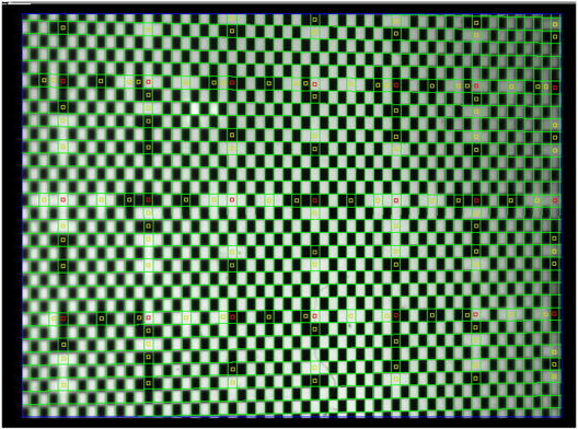
Image skew is caused by one part of the mask being nearer to the lens than the other. In the example above, we have rotated the mask about a vertical axis within the plane of the mask itself, so that the right side is farther away then the left. When the mask is one meter from the lens, the only effect of such rotation is to change the relative sizes of the mask squares in the vertical and horizontal directions. But when the mask is 10 cm from the lens, the skew causes a visible change in square size across the image, and a visible divergence of the mask edges as well.
The x-direction skew is a function of the rotation of the mask about the mask y-axis and the distance from the lens to the image sensor. According to our calculations, we have Sx = tan(α)/b, where α is the rotation and d is the image distance. We also expect α = acos(mx/my), where mx and my are the x and y magnification.
The following derivation shows how image coordinates relate to mask coordinates. We use the suffix p for mask coordinates, because these same calculations apply to any object with a regular pattern of edges. Here we are simplifying our calculation by assuming that the mask is rotated about its y-axis only.
We use the above equation, the assumption that the pattern edges are perpendicular in the image at the pattern origin, as well as the approximation b >> xi to arrive at an expression for the image skew returned by the rasnik analysis.
The skew appears in all coordinate transformations between the pattern and image. We derive the transformation equations for rotation of the mask only about its own y-axis below.
The x and y skew parameters are sufficient to describe the mask image provided the pattern edges are perpendicular at the center of the analysis bounds. In general, however, the pattern edges will not be perpendicular in the image at the pattern origin. The slant of the pattern is the angle by which the pattern x and y directions are less than perpendicular in the image.
The image above has slant −39.13 mrad, x-skew −0.00 mrad/mm, and y-skew −9.83 mrad/mm. The rotation is −11.34 mrad, which is the average rotation of the pattern coordinates at the center of the analysis boundaries. In this case, we see that the angle between the pattern coordinates is 39.13 mrad greater than perpendicular, while the pattern diagonal line is rotated by 11.34 mrad clockwise in the image. Assuming we have corrected for skew and rotation already, the correction for slant will be a linear transformation as derived below.
Image slant can occur even when there is no significant image skew. When we rotate the mask about an axis parallel to its surface but not parallel to either of its coordinate directions, the squares of the mask will appear slanted, regardless of whether or not there is a change in magnification from one side of the image to the other. The squares are being stretched in a direction that is parallel to neither of their edges, and so they become diamond-shaped.
A complete transformation between image and pattern coordinates must account for the offset between the origins of the two systems, magnification in x, magnification in y, rotation within the plane of the image, skew in x, skew in y, the slant. Our hope is that the interactions between these effects are insignificant, so that we can apply the effects sequentially. When we transform from pattern to image coordinates we apply the effect in the order: rotation, magnification, slant, skew, and offset. When we transform from image to pattern coordinates we apply them in the opposite order: offset, skew, slant, magnification, and rotation. We take an ICX424 image with 45° skew and image range 91 mm. We travel along a diagonal line across the pattern coordinate origin and transform image points into pattern points and then back again. We plot the disagreement between the x-coordinate versus x-coordinate along the diagonal.
The error in y is identical when plotted versus x-coordinate. The image extends only to ±350 pixels. The error at the corners of our image area is 0.4 pixels. Even in this extreme example, the average error will be less than 0.1 pixels, which is an error we are willing to accept in return for the computational efficiency of our sequential transformations.
[16-NOV-17] If our rasnik images are rotated by more than 150 mrad with respect to the image sensor rows and columns, the analysis is likely to fail. If we want to analyze a rasnik image that is rotated by 30° or 45°, we rotate the image by −30° or −45° before analysis. We make sure that our analysis bounds enclose only rotated mask squares, and no blank regions introduced by the rotation.
Starting with LWDAQ 8.4.1, the Rasnik Instrument provides the analysis_rotation_mrad parameter in its Info Panel. Use this parameter to specify the nominal rotation of the rasnik pattern in the counter-clockwise direction. The analysis rotates the image clockwise by this angle about the center of the analysis bounds, transforms the reference point into the rotated image coordinates, performs analysis, displays the rotated analysis on the original image, and adds the nominal rotation to the measured rotation to obtain its final result.
We set up a 360-° rotation stand with precision ±0.5 mrad. We mount upon the stand a 30-mm square rasnik mask. We clamp to our table an ICX424AL camera to view the rasnim mask so that the mask image is close to 0° when the stage reads 0°. We rotate the mask by ±50°. At each rotation we set analysis_rotation_mrad to the angle on our stage and capture an image.
We plot the difference between the rasnik-measured rotation and stage rotation.
We choose an ICX424AL image with 45° rotation and vary the pre-rotation constant we use to direct the analysis. We obtain the following plot of measured rotation versus pre-rotation.
So far as we can tell, our error in measuring large rotations is dominated by the error we introduce when we rotate the image in software.
[22-AUG-16] The rotation of the rasnik image we perform with the rotate operation of the lwdaq_image_manipulate routine. To test the accuracy of the rotation algorithm, we use the following code to create a simulated rasnik image with no rotation, rotate the image with the algorithm from −150 mrad to 150 mrad, and apply rasnik analysis.
lwdaq_image_create -width 400 -height 400 -name sim
lwdaq_image_manipulate sim rasnik "200.0 200.0 20.0 20.0 0 10.0 1.0"
catch {image delete p}
image create photo p
destroy $f.i
label $f.i -image p
pack $f.i
for {set rot -150.0} {$rot <= +150.0} {set rot [expr $rot + 10.0]} {
    lwdaq_image_manipulate sim rotate 200 200 [expr $rot/1000.0] -name newimage
    lwdaq_image_manipulate newimage none -left 30 -right 370 -top 30 -bottom 370
    set result [lwdaq_rasnik newimage -pattern_only 1]
    LWDAQ_print $t "$rot $result"
    lwdaq_draw newimage p -intensify exact
    LWDAQ_update
    if {![winfo exists $t]} {break}
}
We obtain the following errors in pattern position. We are subtracting the known, fixed origin position and square sizes from the rasnik analysis measurements of these same parameters. Any offset in the measurement will appear in the graph.
If our pixels are 10μm square, the rotation algorithm introduces less than 0.1 μm error. Errors with a dim, blurred image with significant noise are roughly ten times larger.
[08-AUG-08] We generate rasnik patterns with rotation π/4±0.15 rad in 10-mrad steps. Each image we rotate by −&pi/4 before we apply rasnik analysis. We obtain the rasnik measurement, then rotate by −π/4 to display the results on the screen. Cut and paste the following script into the Toolmaker to reproduce our results.
set wd 400
set ct [expr $wd/2.0]
set nr [expr 3.1415926536/4.0]
set cl 30
lwdaq_image_create -width $wd -height $wd -name sim
catch {image delete p}
image create photo p
destroy $f.i
label $f.i -image p
pack $f.i
for {set rot -30.0} {$rot <= +30.0} {set rot [expr $rot + 2.0]} {
  lwdaq_image_manipulate sim rasnik "$ct $ct 20.0 20.0 [expr $nr*1000 + $rot] 10.0 1.0"
  lwdaq_image_manipulate sim rotate -$nr $ct $ct \
    -name newimage -left $cl -top $cl -right [expr $wd - $cl] -bottom [expr $wd - $cl]
  set result [lwdaq_rasnik newimage -pattern_only 1]
  lwdaq_image_manipulate newimage rotate $nr $ct $ct -name newimage
  lwdaq_image_manipulate sim transfer_overlay newimage
  lwdaq_draw sim p -intensify exact
  LWDAQ_print $t "$rot $result"
  LWDAQ_update
  if {![winfo exists $t]} {break}
}
At rotation π/4−0.06 rad, we see large errors due to confusion over which edge is which. We restrict ourselves to ±30 mrad and obtain the following errors with rotation.
For 10-μm pixels, we will obtain the rasnik measurement to 0.1 μm accuracy even with a nominal rotation of 45°.
[10-AUG-16] When rotating an image, we must make sure the analysis region does not include any of the blank regions introduced by the rotation. We need an automatic way to determine how much to move the analysis boundaries for a given rotation. In the following derivation, we assume that we want the height and width of the boundaries to be reduced by the same amount.
The above formula assumes that the width of the image sensor is greater than or equal to the height, and that the rotation angle is greater than zero. If the height is greater than the width, we reverse the role of width and height in the formula. If the angle is negative, we take its absolute value. The graph below shows how far we must move the analysis borders for various image sensor dimensions and rotations.
Our ICX424 image, when rotated by 45° requires that we bring in all the borders by 114 pixels, which reduces the width of the analysis bounds from 658 to 430 and the height from 492 to 264.
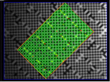
We apply analysis to image Rasnik_blurred.gif image, which we keep in the image library we bundle with LWDAQ. We vary analysis_rotation_mrad from −150 to 150 mrad in 1-mrad steps. At 150 mrad, we get the following display of results.
The orange rectangle is the analysis bounds used in the rotated image where analysis takes place. For each nominal rotation, we are rotating the image prior to analysis. With the image above, the standard devition of x is 1.0 μm and of y is 1.6 μm. The standard deviation of rotation is 2 mrad. We apply rasnik analysis with nominal rotation 0 mrad and 50 mrad to 552 images from the ATLAS End-Cap Alignment System. The standard deviation of the difference in x and y is 1.0 μm and in rotation is 0.5 mrad. (Also, when we cmompare LWDAQ 7.9.6 and LWDAQ 8.4.1 with 0 mrad, the results are identical.)
[20-MAY-24] At the bottom of rasnik.pas is a routine called rasnik_analyze_image.
function rasnik_analyze_image(ip:image_ptr_type;
	orientation_code:integer;
	reference_x,reference_y,square_size_um,pixel_size_um:real):rasnik_ptr_type;
The routine takes six parameters. The first, ip, is a pointer to an image_type structure. We describe the image_type and all other structures defined by our code in the Data Types section below. The image_type contains a two-dimensional array of eight-bit gray-scale pixels, as well as auxiliary information about the image.
The orientation_code parameter tells rasnik_analyze_image the true orientation of the mask. Here are the values of orientation_code defined in rasnik.pas.
rasnik_mask_orientation_nominal=1;
rasnik_mask_orientation_rotated_y=2;
rasnik_mask_orientation_rotated_x=3;
rasnik_mask_orientation_rotated_z=4;
rasnik_try_all_orientations=0;
The square_size parameter gives the size of the squares in the rasnik mask. We assume they are square, not rectangular. Likewise, the pixel_size parameter gives the size of the pixels in the image sensor.
The rasnik_analyze_image procedure returns a rasnik_ptr_type, which is a pointer to a newly-created rasnik_type structure. The rasnik_type contains the results of rasnik analysis, as well as the input parameters, but not the image_type itself. There is enough information in the rasnik_type for us to re-calculate the rasnik measurement with respect to a different reference point, using a routine like rasnik_shift_reference_point. We describe the fields of the rasnik_type in the next section.
The body of rasnik_analyze_image is a sequence of subroutines.
iip:=image_grad_i(ip);
jip:=image_grad_j(ip);
These two routines create two more images giving us the absolute value of the intensity derivative in the horizontal (i) and vertical (j) directions, as we describe above. Both routines operate upon an image_type and return a new image_type. You will find the routines defined in image_manip.pas. The derivative images show the horizontal and vertical edges in the image.
pp:=rasnik_find_pattern(iip,jip,false);
This step finds the approximate pattern using slices of the derivative images, one-dimensional fourier analysis (see above), and smoothing of the intensity profile (see above). The routine takes as input the two derivative images and a show_fitting flag. When true, this flag instructs the routine to show stages of analysis via the graphical user interface. The routine returns a pointer to a new rasnik_pattern_type structure, which defines the phase, period, and rotation of a chessboard pattern overlayed upon the image. We describe the rasnik_pattern_type in the next section.
rasnik_refine_pattern(pp,iip,jip,false);
This step refines the approximate pattern by fitting lines to edge pixels (see above). The routine operates upon an existing rasnik_pattern_type pointed to by pp.
rasnik_adjust_pattern_parity(ip,pp);
So far, the analysis has looked only at edges in the image. It has determined the orientation and magnification of the rasnik pattern, and determined a viable offset for this pattern that will place its edges in the correct place on the two derivative images. But the analysis has not yet made sure that the white squares of its pattern coincide with the white squares in the image. The rasnik_adjust_pattern_parity routine looks at the original image, as pointed to by ip, and adjusts the pattern, as pointed to by pp, so that the white squares in the pattern match the white squares in the image.
rasnik_identify_pattern_squares(ip,pp);
This step is the first to use of the squares field of the rasnik_pattern_type pointed to by pp. The squares field is a two-dimensional array with an element for each square of the pattern. The routine marks the squares in the squares array that correspond to squares in the image that lie within the image's analysis boundaries.
rasnik_identify_code_squares(ip,pp);
This steps marks the squares in the squares array that are out of parity in the image. The out of parity squaresa are the rasnik code squares. The routine marks as pivot squares any code squares that are at the intersection of lines and columns of code squares.
rasnik_analyze_code(pp,orientation_code);
This step analyses the squares array the rasnik_pattern_type pointed to by pp. It records records the line and column codes of each valid pivot squares. The orientation_code parameter tells the analysis whether it should guess the orientation or use a particular orientation.
rp:=rasnik_from_pattern(ip,pp,reference_x,reference_y,square_size_um,pixel_size_um);
The rasnik_from_pattern routine takes the pattern pointed to by pp, which has all its pivot squares marked with their line and column codes, and calculates the final rasnik measurement. It stores the measurement in a new rasnik_type structure and returns a pointer to that structure. The referencde_x and reference_y parameters are used only when the reference_code is equal to the value rasnik_reference_image_point. We need to pass ip to this routine because we need to know the dimensions of the image and its analysis bounds for various values of reference_code.
dispose_rasnik_pattern(pp);
dispose_image(iip);
dispose_image(jip);
These steps free up the memory used by the pattern and the derivative images.
rasnik_analyze_image:=rp;
The final step is to return a pointer to the rasnik_type that contains the rasnik measurement. This rasnik_type structure was allocated dynamically, so the calling procedure must call dispose_rasnik to de-allocate the structure.
[20-MAY-24] If you want to link our rasnik analysis routines directly to your own code, we provide a shared library for your convenience. To create the shared library, install GNU Make and the FPC on your machine, navigate to the LWDAQ repository's Build directory, and type "make analysis". Your machine will build a native analysis dynamic libarary. It will be named "libanalysis.dylib" on MacOS, "analysis.dll" on Windows, and "libanalysis.so" on Linux. Examine analysis.pas for a list of routines exported by the shared library.
The analysis library exports its functions in the standard C calling convention, which we specify with the FPC "cdecl" compiler directive. So long as your own import routines use the same convention, you will be able to link and call the LWDAQ analysis routines. But you will need to know structure of the various data types used by our Pascal routines. The rasnik_analyze_image function, for example, uses three data types for its input parameters: image_ptr_type, integer, and real. It returns a pointer to a newly-allocated rasnik_type. Inside rasnik_analyze_image, we see a rasnik_pattern_type used by several stages of the analysis. Type the command "make test" in the Build directory to create a test executable that will not only test the functionality of a variety of our analysis routines on your native platform, but also print out for you the sizes of a selection of its data types.
In our code, an integer is a four-byte signed value, as dictated by a type declaration at the top of utils.pas. A real is an eight-byte floating-point number. An xy_point_type is a pair of real-valued coordinates, defined in utils.pas. We also have ij_point_type, which is a pair of integer-valued coordinates. We have ij_rectangle_type to represent a rectangle in an image. It contains four integers.
A byte is an unsigned eight-bit integer, value 0 to 255. A boolean is a binary variable. A solitary boolean can be stored in as little as one bit in memory. We could fit eight into a single byte. By default, we do not pack our variables into their structured types. We allow them to be placed by the compiler on the boundaries natural to the native architecture. On a sixty-four bit machine, booleans will be placed on eight-byte boundaries. On a thirty-two bit machine, they will be on four-byte boundaries. We make an exception, however, for two-dimensional arrays of pixels in images, and in one-dimensional graphical arrays. In these cases, we pack the values so as to reduce their space and increase the efficiency with which we can copy the arrays.
Our short_string and long_string types are defined in utils.pas as being 255 and 300k characters long. A Pascal string is similar to a C string, but instead of being null-terminated, it has a length parameter. To translate between Pascal strings and C strings, our analysis library uses FPC's "PChar" type, which performs the translation automatically.
The first input to rasnik_analyze_image is an image_ptr_type, which is a pointer to an image_type. The image_type is defined in image.pas. An image_type's discriminants are the number of lines, j_size, and the number of columns, i_size you see in the image_type definition below.
image_type=record
	i_size,j_size,intensification:integer;
	intensity:packed array of intensity_pixel_type;
	overlay:packed array of overlay_pixel_type;
	analysis_bounds:ij_rectangle_type;
	average,amplitude,maximum,minimum:real;
	name,results:string;
end;
image_ptr_type=^image_type;
We specify j_size and i_size when we creat a new image_type. We create an image_type with the following Pascal instruction.
ip:=new_image(j_size,i_size);
In this Pascal instruction, the ip variable is a pointer to an image_type, which we call an image_ptr_type. The number of rows in the image is j_size, and the number of columns is i_size. In our code, we tend to use j and i to indicate row and column number respectively.
There are two pixel arrays in an image_type. The intensity array contains the pixels of the image. In the current version of our code, these pixels are each one-byte gray-scale intensities. The overlay array has the same dimensions as the intensity array. Each overlay pixel is also one byte.
The overlay contains a picture, graph, or set of marker lines that we draw on top of the intensity when we display the image for the user. When overlay[j,i] is not equal to clear_color, we change the color of pixel intensity[j,i] in the image display. The color with which we draw overlay[j,i] depends upon its value. You will find a list of colors and their corresponding values in image.pas. The ranik routines draw into the overlays of the original image and the derivative images, and so make it possible for our LWDAQ Software to display the results and stages of anlysis in such a way that we can spot problems and make corrections.
The analysis_bounds field is an ij_rectangle_type that defines a rectangle in the image within which image analysis is to take place. Pixels outside the analysis_bounds will be ignored. The ij_rectangle_type is defined in utils.pas as follows:
ij_rectangle_type=record top,left,bottom,right:integer; end;
The average, amplitude, maximum, and minimum fields are real numbers. We use these variables to store properties of the image during certain image analysis procedures. But we do not use them in rasnik analysis.
The name field holds a name for the image, which we use to organise and sort the LWDAQ Software's internal image list. The intensification field selects one of sevaral types of intensification available for screen display of the gray-scale image.
no_intensify=0;
mild_intensify=1;
strong_intensify=2;
exact_intensify=3;
The results field is a string we use to pass data acquisition parameters to certain image analysis routines. The only use our rasnik analysis makes of any of these three fields is to use the name field when setting up its diagnostic displays.
The result returned by rasnik_analyze_image is a pointer to a rasnik_type, defined in rasnik.pas as follows.
rasnik_type=packed record
	valid:boolean;{no problems encountered during analysis}
	padding:array [1..7] of byte;{force mask_point to eight-byte boundary}
	mask_point:xy_point_type;{point in mask, um}
	magnification_x,magnification_y:real;{magnification along pattern coords}
	skew_x,skew_y:real;{skew in x and y directions in rad/m}
	slant:real;{radians non-perpendicularity in image}
	rotation:real;{radians anticlockwize in image}
	error:real;{um rms in mask}
	mask_orientation:integer;{orientation chosen by analysis}
	reference_point_um:xy_point_type;{point in image, um from top-left corner}
	square_size_um:real;{width of mask squares}
	pixel_size_um:real;{width of a sensor pixel in um}
end;
We have already defined each of the simple types used in the rasnik_type structure. Because the rasnik_type consists only of fixed-length fields, it is possible to pass a rasnik_type directly from Pascal to C or Fortran. But we must make sure our compilers agree upon how to arrange the structure fields in memory. The offset of each field from the base address of the rasnik_type is given by the following table.
| Field | Type | Offset |
|---|---|---|
| valid | boolean | 0 |
| padding | byte array | 1 |
| mask_point | xy_point_type | 8 |
| magnification_x | real | 24 |
| magnification_y | real | 32 |
| skew_x | real | 40 |
| skew_y | real | 48 |
| slant | real | 56 |
| rotation | real | 64 |
| error | real | 72 |
| mask_orientation | integer | 80 |
| reference-point | xy_point_type | 84 |
| square_size_um | real | 100 |
| pixel_size_um | real | 108 |
The padding field ensures that all four-byte variables are on four-byte boundaries, and all eight-byte variables are on eight-byte boundaries. We do this because the newer versions of GPC will place the eight-byte variables on eight-byte boundaries whether we like it or not. The only way for our rasnik_type to be compatible with all versions of GPC and GCC is to force the eight-byte variables onto eight-byte boundaries regardless of the compiler.
The intermediate stages of rasnik analysis, as described above use a rasnik_pattern_type structure to store information about the image and the rasnik pattern.
rasnik_pattern_type=packed record {based upon pattern_type of image_types}
	valid:boolean;{most recent analysis yielded valid output}
	padding:array [1..7] of byte;{force origin to eight-byte boundary}
	origin:xy_point_type;{pattern coordinate origin in image coordinates}
	rotation:real;{radians anticlockwize wrt image coords}
	pattern_x_width,pattern_y_width:real;{square width in pixels along pattern coords}
	image_x_skew,image_y_skew:real;{derivative of line slope in rad/pixel}
	image_slant:real; {non-perpendicularity of pattern in image in rad}
	image_x_width,image_y_width:real;{square separation in pixels along image coords}
	error:real;{pixels rms in image}
	extent:integer;{extent of pattern from center of analysis bounds}
	mask_orientation:integer;{integer indicating orientation of mask}
	x_code_direction,y_code_direction:integer;{directions of code increment}
	analysis_center_cp:ij_point_type;{ccd coords of analysis bounds center}
	analysis_width:real;{diagnonal width of anlysis bounds}
	squares:rasnik_square_array_ptr_type;{array of rasnik squares}
	more_padding:array [1..4] of byte;{force end to eight-byte boundary}
end;
As with rasnik_type, the padding field makes sure that all the eight-byte variables are on eight-byte boundaries. Here are the address offsets of each field.
| Field | Type | Offset |
|---|---|---|
| valid | boolean | 0 |
| padding | byte array | 1 |
| origin | xy_point_type | 8 |
| rotation | real | 24 |
| pattern_x_width | real | 32 |
| pattern_y_width | real | 40 |
| pattern_x_skew | real | 48 |
| pattern_y_skew | real | 56 |
| image_x_width | real | 64 |
| image_y_width | real | 72 |
| image_slant | real | 80 |
| error | real | 88 |
| extent | integer | 92 |
| mask_orientation | integer | 96 |
| x_code_direction | integer | 100 |
| y_code_direction | integer | 104 |
| analysis_center_cp | ij_point_type | 108 |
| analysis_width | real | 116 |
| squares | rasnik_square_array_ptr_type | 124 |
| more_padding | byte array | 128 |
The squares field is a pointer to a two-dimensional array of rasnik_square_type structures. This array contains an element for every square in the rasnik image, and allows every square to be classified as black or white, as a code square, as as a pivot square. We describe the the rasnik_square_type below, and the rasnik_square_array_type also.
The rasnik_find_pattern routine creates a new pattern_type with our new_rasnik_pattern routine. It fills in the valid, origin, rotation, pattern_x_width, pattern_y_width, image_x_width, image_y_width, and extent fields for use in subsequent routines like rasnik_refine_pattern and rasnik_adjust_pattern_parity.
A rasnik_square_type describes a single square in a rasnik pattern.
rasnik_square_type=packed record
	center_pp:xy_point_type; {center of square in pattern coordinates}
	center_intensity:real; {average intensity of central region}
	center_whiteness:real; {whiteness score, >0 for white, <=0 for black}
	pivot_correlation:integer; {number of agreeing pivot squares}
	x_code,y_code:integer; {the column and line codes for the pivot square}
	display_outline:ij_rectangle_type; {a rectange for square marking}
	is_a_valid_square:boolean; {within the analysis boundaries}
	is_a_code_square:boolean; {out of parity with the chessboard}
	is_a_pivot_square:boolean; {at intersection of code line and column}
	padding:array [1..13] of byte; {ample padding to eight-byte boundary}
end;
The rasnik_square_type uses an array of bytes to pad its size to an eight-byte boundary. In fact, we leave a little extra padding to accomodate additional fields in the future.
| Field | Type | Offset |
|---|---|---|
| center_pp | xy_point_type | 0 |
| center_intensity | real | 16 |
| center_whiteness | real | 24 |
| pivot_correlation | integer | 32 |
| x_code | integer | 36 |
| y_code | integer | 40 |
| display_outline | ij_rectangle_type | 44 |
| is_a_valid_square | boolean | 60 |
| is_a_code_square | boolean | 61 |
| is_a_pivot_square | boolean | 62 |
| padding | array of bytes | 63 |
We use the rasnik_square_type to form the elements of the array pointed to by the squares pointer in a rasnik_pattern_type.
A rasnik_square_array is a dynamically-allocated two-dimensional array of rasnik_square_type elements. The array provides an element for each square in a rasnik image. When we create the array, we specify its dimensions with the extent discriminant.
rasnik_square_array_type(extent:integer)=
    array [-extent..extent,-extent..extent] of rasnik_square_type;
When we first create a rasnik_pattern_type, the squares pointer is set to nil. The routine rasnik_identify_pattern_squares creates a two-dimensional array of rasnik_square_type just large enough to cover the rasnik squares in the image. A typical square array will have extent 19 and contain 1600 squares, each of size 80 bytes. The total array is 128 kBytes. But some rasnik images contain tiny squares, and our extent can be up to 39, in which case our array size is 512 kBytes.
[22-DEC-17] Our code uses three coordinate systems. We call them ccd, image, and pattern coordinates. Our transforms.pas unit defines the three coordinate systems and declares routines to transform between them.
Our ccd coordinates specify a pixel in an image. They are named after the type of image sensor we used for most of our cameras. The letters CCD stand for Charge-Coupled Device. Our CCD images are rectangular with square pixels. The pixels are arranged in rows and columns. We specify a pixel in the image with its column and row number. A ccd point has the form (i,j) where i is the column number and j is the row number. Pixel (0,0) is the top-left pixel. Column number increases from left to right and row number increases from top to bottom. CCD Coordinates are therefore left-handed. We use ij_point_type for points in CCD Coordinates. You will find ij_point_type defined in our utils unit. Our image coordinates specify a point in an image. An image point has the form (x,y), where x and y are real numbers, x is horizontal distance from left to right and y is vertical distance from top to bottom. The units of both x and y are pixels. Image point (0,0) is at the top-left corner of the top-left pixel. Point (1,1) is the bottom-right corner of the top-left pixel, and also the top-left corner of the second pixel in the second row. We have constants ccd_origin_x and ccd_origin_y that define the location of the ccd coordinate origin in image coordinates. The values declared in our current version of rasnik.pas are 0.5 and 0.5, which places the ccd origin at the center of the top-left pixel. Our pattern coordinates specify a point in a pattern superimposed on an image. Pattern points are ot the form (x,y), where x and y are the real. We assume the pattern is periodic in two orthogonal directions. A chessboard rasnik mask is such a pattern, and so is a sequence of encoder lines. The chessboard has a finite period in two directions, while the encoder lines have a finite period in one direction and a large period in the other direction. The x-axis is parallel to one direction in the orthogonal pattern, and the y-axis is parallel to the other direction. Pattern coordinates are left-handed for better cooperation with ccd and image coordinates, both of which are left-handed. We define a pattern coordinate system with five numbers grouped in a pattern_type record. These numbers represent a translation, rotation, and scaling in two directions between image coordinates and pattern coordinates.pattern_type=record
valid:boolean;{valid pattern}
origin:xy_point_type; {pattern coordinate origin in image coordinates}
rotation:real; {radians}
pattern_x_width:real; {scaling factor going from pattern x to image}
pattern_y_width:real; {scaling factor going from pattern y to image}
image_x_skew:real; {derivative of horzontal edge slope with x in rad/pixel}
image_y_skew:real; {derivative of vertical edge slope with y in rad/pixel}
image_slant:real; {non-perpendicularity of pattern x and y in image in rad}
end;
The pattern_type structure matches that of the first few fields of the rasnik_pattern_type. The origin field is an xy_point_type that gives the image coordinates of the pattern coordinate origin. The origin will have some significance in the pattern. In the case of rasnik analysis, the origin lies at the top-left corner of a chessboard square. In our wire-finding code, the origin lies at the center of a wire shadow. We choose the origin square so that the pattern coordinate origin is near the center of the analysis bounds. This choice minimizes the errors that arise from rotation and skew in the image. The rotation field gives the rotation of the pattern coordinates in the anticlockwise direction with respect to image coordinates. The pattern_x_width field gives the length of one period of the pattern along the pattern x-axis, as measured in image coordinates. Imagine the pattern x-axis inclined at a slight angle with respect to the image rows, and therefore to the image x-axis. A square in the pattern has one edge parallel to the pattern x-axis. The length of this edge, as measured in the image coordinates, is pattern_x_width. We have pattern_y_width as well, because a pattern can, in general, be rectangular in its geometry.
We assume the mask itself contains perfect, uniform, squares. But the projection of the mask onto the image sensor can be both skewed and stretched. If the mask is rotated about its x-axis, for example, the squares will appear narrower in the x-direction than in the y-direction. Our pattern accounts for this difference with its two values of pattern width. If the distance from the mask to the lens is such that the rotation causes a significant change in the opject distance of the mask across the image, the width and height of the squares will change across the image. Our pattern accounts for this variation with its two skew parameters.
The pattern coordinate origin is the top-left corner of the origin square in a chessboard pattern. Point (1,0) marks the top-right corner of the same square, and also the top-left corner of the square to its right. Here were defining right and left as +ve and −ve in the x-direction, and top and bottom as +ve and −ve in the y-direction. Point (0,1) is the bottom-left corner of the same square, and the top-left corner of the square immediately below. Moving around through a chessboard pattern is easy in pattern coordinates, because we simply add one to our x-coordinate to move to the square on the right, and add one to our y-coordinate to move to the square below. Transforming between image and pattern coorsinates is more complicated, because of the asymmetry, rotation, skew, and slant between the image and the object. Here are the two routines we use to move between the two coordinate systems. For a derivation of the effecty of skew upon the transform, see Skewed Images.function p_from_i(point:xy_point_type;pattern_ptr:pointer):xy_point_type; const min_slant_cosine=0.5; var p:pattern_ptr_type;q,r:xy_point_type;slant,c,s,cc:real; begin p:=pattern_ptr_type(pattern_ptr); with p^ do begin q.x:=(point.x-origin.x); q.y:=(point.y-origin.y); r.x:=q.x/(1 + image_x_skew*q.x)/(1 + image_y_skew*q.y); r.y:=q.y/(1 + image_x_skew*q.x)/(1 + image_y_skew*q.y); if slant>max_slant then slant:=max_slant; c:=cos(image_slant/2); s:=sin(image_slant/2); cc:=c*c-s*s; q.x:= (c*r.x - s*r.y)/cc; q.y:= (-s*r.x + c*r.y)/cc; r.x:=q.x/pattern_x_width; r.y:=q.y/pattern_y_width; c:=cos(rotation); s:=sin(rotation); q.x:=r.x*c - r.y*s; q.y:=r.x*s + r.y*c; end; p_from_i:=q; end; function i_from_p(point:xy_point_type;pattern_ptr:pointer):xy_point_type; var p:pattern_ptr_type;q,r:xy_point_type;slant,c,s:real; begin p:=pattern_ptr_type(pattern_ptr); with p^ do begin c:=cos(rotation); s:=sin(rotation); q.x:= point.x*c + point.y*s; q.y:= -point.x*s + point.y*c; r.x:=q.x*pattern_x_width; r.y:=q.y*pattern_y_width; if slant>max_slant then slant:=max_slant; c:=cos(image_slant/2); s:=sin(image_slant/2); q.x:= c*r.x + s*r.y; q.y:= s*r.x + c*r.y; r.x:=q.x /(1 - image_x_skew*q.x) *(1 + image_y_skew*q.y/(1 - image_y_skew*q.y)) + origin.x; r.y:=q.y /(1 - image_y_skew*q.y) *(1 + image_x_skew*q.x/(1 - image_x_skew*q.x)) + origin.y; end; i_from_p:=r; end;The pattern_type is the basis of any record used with the pattern coordinate tranform routines defined in this unit. But the pattern_type is not public. All transform routines refer to patterns through generic pointers. When another unit declares its own pattern record for use with the routines declared in this unit, the new record must begin with the same fields as pattern_type, so these fields may be referred to through a pointer as if the new record were a genuine pattern_type. See rasnik_pattern_type in rasnik.pas for an example of such a pattern type.
The rasnik_pattern_type places its pattern coordinate origin at the top-left corner of a rasnik square. Any rasnik square will do, but our analysis tries to pick one that's near the center of the image. If p is a rasnik_pattern_type, the point (0,0) in pattern coordinates lies at point p.origin in image coordinates. Just to be clear, we'll say the same thing again: the origin field is an xy_point_type giving the image coordinates of the pattern coordinate origin. The rotation field gives the rotation of the pattern x-axis with respect to the image x-axis, with counter-clockwise rotation being positive. The pattern_x_width parameter is the distance between pattern points (0,0) and (1,0) after they have been transformed into image coordinates. When the pattern rotation is small, pattern_x_width gives the length of the near-horizontal sides of the squares. The pattern_y_width parameter is the length of the near-vertical sides of the squares.
You can write your own routine to find the rasnik pattern in an image, and make use of our code square analysis afterwards. Several people have done this, having decided that their pattern-finding routine is superior to ours, or simply as a means of comparing several pattern-finding routines. To implement your own pattern-finding routine, give it the same structure and output as our rasnik_find_pattern routine. Create a new pattern_type and fills the following fields: valid, origin, rotation, pattern_x_width, pattern_y_width, image_x_width, image_y_width, and extent. You may now pass this pattern_type to our rasnik_refine_pattern, where it will be refined, or you can skip our refining routine and go straight to rasnik_adjust_pattern_parity and proceed all the way through code square analysis to rasnik_from_pattern.
[10-DEC-08] We receive a report from Rikard Sandstrom at CERN that our magnification measurements are in error when the mask is rotated. Harry van der Graaf of NIKHEF produced a library of simulated images with rotation from -100 mrad to +100 mrad. Unlike our own simulated images, these images contain code square markings. You will find them in NIKHEF_Images.zip. Rikard sent us a graph of our magnification error versus image number and compared to the magnification error from the FOAM and FORTRAN rasnik analysis programs. It turns out that we broke our magnification calculation back in late 2007. Instead of multiplying by cos(rotation) in several places, we were dividing by cos(rotation). We fixed the bug and Rikard obtained another graph in which the error looks similar to the one we obtain ourselves.
We analyzed the NIKHEF images ourselves with LWDAQ 7.3.20 with the following Tcl script, which we executed in our Toolmaker.
upvar #0 LWDAQ_config_Rasnik iconfig
upvar #0 LWDAQ_info_Rasnik iinfo
set iconfig(analysis_enable) 3
set iconfig(analysis_reference_code) 3
set iinfo(analysis_min_width) 250
set iconfig(image_source) file
LWDAQ_open Rasnik
set d [LWDAQ_get_dir_name]
set fl [glob -nocomplain [file join $d *.gif]]
set fl [lsort -dictionary $fl]
foreach  f $fl {
  set LWDAQ_config_Rasnik(file_name) $f
  set result [LWDAQ_acquire Rasnik]
  LWDAQ_print $t $result
  LWDAQ_support
  if {![winfo exists $t]} {break}
}
We obtained the following graph of magnification and position deviation with rotation.
The rotation in these patterns appears to take place about the top-left corner of the image instead of the center. Our position measurement is therefore coupled to our rotation measurement. It may be this coupling that gives us inferior position results compared to those we obtained with our own simulated images. Our own images rotate about the center of the image.
[31-MAY-24] We encounter Rasnik_contact, a contact print rasnik image that thwarts the Fourier transform algorithm we use to obtain our first estimate of the square size. We update our pre-filters: we smooth after shrinking. We are able to analyse Rasnik_contact with ×3 or ×4 shrinking.